Introducing Interpretable Machine Learning and(or) Explainability
Gone are the days when Machine Learning models were treated as black boxes. Therefore, as Machine Learning gets mainstream, accountability for the models will increase. Hence, explainability and (or) interpretability for ML models is gaining a lot of traction. But first things first. What is the difference between Interpretability and Explainability? Interpretability is the ability to interpret the association between the input and output. Explainability is the ability to explain the model’s output in human language. In this article, we will talk about the first paradigm viz. Interpretable Machine Learning.
Interpretability stands on the edifice of feature importance. However, not all ML models are interpretable. Even if they are interpretable, they provide global feature importance. Now, what on earth is global feature importance? Logically, is there a concept of local interpretability? Let’s walkthrough.
Global Feature Importance
Global Feature Importance quantifies the importance of each feature for prediction in the overall dataset. For example, the impact of Sepal Length to predict species in the entire IRIS dataset is the global feature importance of Sepal Length. Certain models like Linear and Logistic Regression, Decision Trees, Naive Bayes and KNN, etc provide global feature importance.. However, Global feature importance gives the overall feature importance on the test data set. What if we want interpretability for a particular datapoint? The answer is Local Feature Importance.
Local Feature Importance
Local feature importance is the measure of influence of a feature on an individual data point prediction. For example, the impact of Sepal Length on the prediction of species for a particular instance of a flower is the local feature importance of Sepal Length. So how do we get local feature importance if all the models give global importance? Two techniques have emerged to the forefront viz. LIME and SHAP.
LIME : Local Interpretable Model-Agnostic Explanations
This is an algorithm that can explain the predictions of any model by approximating it locally with an interpretable model. Hence, this technique creates a surrogate model in the neighbourhood of the point under consideration. To understand the intuition, let’s take an illustration from the Lime Research Paper:
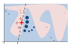
In the above image, the blue region represents the class blue. Likewise, pink region represents class pink. As one can see, a complex decision boundary is fit by a non-linear model, like kernel SVM or Random Forest or any ensemble.
Now, if we seek an explanation for the bold ‘+’ point in red, the dotted line is the surrogate interpretable model, which can give feature importance. The mathematics of this technique is beyond the article. Here is the link to the original paper. In this article, we bring Interpretable Machine Learning hands-on.
Step 0: Install Lime
We install LIME as a step zero:
pip install lime
Step 1: Load Data
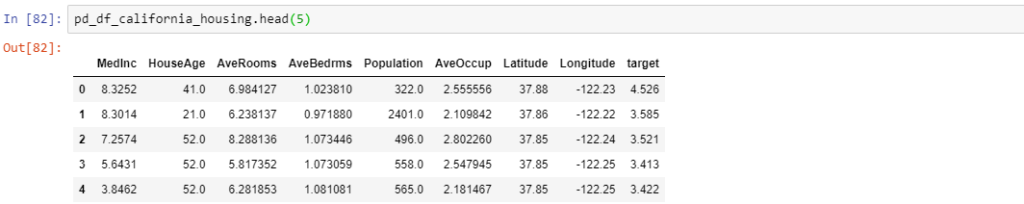
In the first step, we import the data. We use California Housing Data, which is a regression dataset. This dataset has eight features and label named target. Here are the details about the features. The target is the price of the house in 100 thousand dollars. Following is the list of features and the label:
- MedInc – Median income in block group in hundred thousand dollars.
- HouseAge – Median house age in block group.
- AveRooms – Average number of rooms per household.
- AveBedrms – Average number of bedrooms per household.
- Population – Block group population.
- AveOccup – Average number of household members.
- Latitude – Block group latitude.
- Longitude – Block group longitude.
- target – Price of the house in hundred thousand dollars.
Here is the code:
import lime
import shap
import pandas as pd
from sklearn.datasets import fetch_california_housing
Further, let’s load the data into a pandas dataframe:
california_housing = fetch_california_housing()
pd_df_california_housing = pd.DataFrame(california_housing.data, columns = california_housing.feature_names)
pd_df_california_housing['target'] = pd.Series(california_housing.target)
Step 2: Train-Test Split
Next, we separate the label and features:
y = pd_df_california_housing['target'].values
X = pd_df_california_housing.drop(['target'], axis=1)
Further, we split the label and features into train, test, and cross validation datasets:
from sklearn.model_selection import train_test_split
X_train, X_test, y_train, y_test = train_test_split(X, y, test_size=0.30)
X_train, X_cv, y_train, y_cv = train_test_split(X_train, y_train, test_size=0.30)
Step 3: Hyperparameter Tuning
For demonstration purpose, we will train a complex model like XgBoost. However, to have an optimal model, we need to find the best parameters for the same. Here, we use the parameters n_estimators and max_depth. Moreover, we will use simple cross validation for tuning these hyper-parameters with the below code snippet:
import xgboost as xg
from sklearn.metrics import r2_score

n_estimators = [50,100,200,500,1000]
max_depth = [5, 10]
cv_r2_score_array = []   #R2 Score array for different values.

for i in n_estimators:
    for j in max_depth:

    print("for n_estimators =", i,"and max depth = ", j)

    xgb = xg.XGBRegressor(n_estimators=i, max_depth=j,random_state=0)
    xgb.fit(X_train, y_train)
    y_pred = xgb.predict(X_cv)

    cv_r2_score_array.append(r2_score(y_cv, y_pred))

    print("R2_score :",r2_score(y_cv, y_pred))
It was found that the best R2 score was 0.8309, for n_estimators =200 and max_depth=5.
Step 4: Train and test the model
With the best parameters, train the model and evaluate it:
xgb = xg.XGBRegressor(n_estimators=200, max_depth=5,random_state=0)

xgb.fit(X_train, y_train)
y_pred = xgb.predict(X_test)
test_r2_score = r2_score(y_test, y_pred)
The test R2 score was found to be 0.827.
Step 5: Setup Lime Explainer
LIME explainers come in multiple flavours based on the type of data that we use for model building. For instance, for tabular data, we use lime.lime_tabular method. Similarly, we can use lime.lime_text for text data and lime.lime_image for images. For our case, we will use the first one. Here is how we define the explainer:
from lime import lime_tabular

explainer = lime_tabular.LimeTabularExplainer(
training_data=np.array(X_train.values),
feature_names=X_train.columns,
mode='regression'
)
Step 6: Generate Explanations
Once the explainer is built, we generate explanations for a particular test data point. Let’s take the data point number 1001 from the test dataset. The ground truth value/target for this point is 4.163, i.e. ~ 416 thousand dollars and the predicted value is 4.74 ie. ~474 thousand dollars.
Here is the code for generating explanations:
exp = explainer.explain_instance(
data_row=X_test.iloc[1000].values,
predict_fn=xgb.predict
)

exp.show_in_notebook(show_table=True)
The explanations generated are:
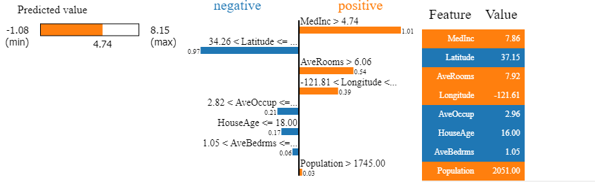
As we can see here, the predicted value is 4.74. We can see that for this datapoint, the biggest influence is MedInc i.e. median income. It influences the price to a higher side. However, the latitude does the opposite. But again, the number of rooms and longitude are a positive influence.
SHAP: SHapely Additive exPlanations
LIME has certain limitations viz. lack of robustness. The biggest limitation is the vague definition of neighbourhood and the kernel width. To know more about this, refer to this link.
This lack of robustness is overcome by SHAP, which is a game theoretic approach. It provides mathematical guarantees by using all the models trained with every combination of features. The difference between Permutation features importance and SHAP is that the former uses error in prediction while the latter uses feature contribution. For details, read this. Having said that, mathematics of SHAP is beyond this article. For a deeper intuition, here is an article.
As far as the demo is concerned, the first four steps are the same as LIME. However, from the fifth step, we create a SHAP explainer. Similar to LIME, SHAP has explainer groups specific to type of data (tabular, text, images etc.)
However, within these explainer groups, we have model specific explainers. For instance, for tree based models, we have TreeExplainers. For more details, refer to this link. Now, let’s get into the code:
exp = shap.TreeExplainer(xgb)   #Tree Explainer
shap_values = exp.shap_values(X_test)  #Calculate Shap Values
shap.initjs()
Global Explanations/Feature importance
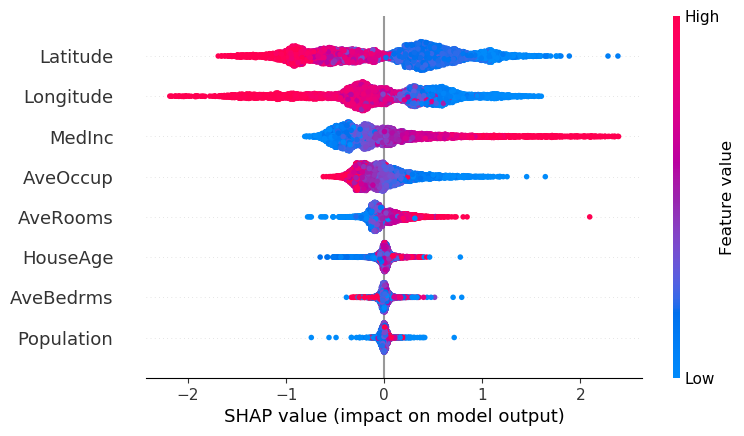
Please note here that SHAP can calculate the Global Feature Importances inherently, using summary plots. Hence, once the shapely values are calculated, it’s good to visualize the global feature importance with summary plot, which gives the impact (positive and negative) of a feature on the target:
shap.summary_plot(shap_values, X_test)
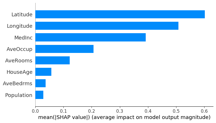
We can plot this as a bar plot to get the mean of absolute values of the feature importance:
shap.summary_plot(shap_values, X_test,plot_type="bar")
Local Explanations
Local explanations with SHAP can be displayed with two plots viz. force plot and bar plot. Let’s take the same 1001th plot.
A force plot is a visual that shows the influence of feature(s) on the predictions:
shap.force_plot(exp.expected_value, shap_values[1000],features =X_test.iloc[1000,:] ,feature_names =X_test.columns)
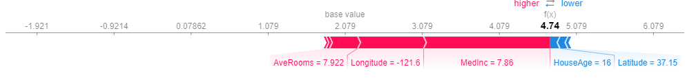
The red arrowed features push the target higher while the blue ones drag the target to the contrary. We can see that the Median Income forces the predicted value to the higher side.
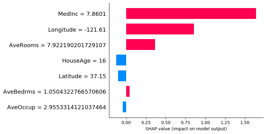
Another way in which we can display is a bar plot:
shap.bar_plot(shap_values[1000],features =X_test.iloc[1000,:] ,feature_names =X_test.columns )
LIME vs SHAP
Lastly, here is a comparison table between two techniques:
| Criteria | LIME | SHAP |
| Speed | Fast | Slow(except for Tree Explainer) |
| Robustness | Less Robust | Robust Mathematical Guarantees |
| Local/Global Explanations | Inherently Local(SP LIME for global) | Both Global and Local Interpretability |
Conclusion
We hope this article on Interpretable Machine Learning is useful and intuitive. Please note that this is for information only. We do not claim any guarantees regarding the code, data, and results. Neither do we claim any guarantees regarding its accuracy or completeness.
As a parting note, Interpretable Machine Learning is a part of Responsible AI triad. To know more about Responsible AI triad (RAI Triad) and its first tenet viz. Privacy, read this article: A look at Differential Privacy