A look at Differential Privacy

AI is a superpower. And with power comes responsibility. This takes us into the domain of Responsible AI.

In 2016, Microsoft released a bot named Tay on Twitter. However, over time, it started posting inflammatory speeches, causing a stir. We have heard of instances when AI agents discriminated against users based on race, gender, ethnicity, etc. Thus, in this age of AI empowerment, Responsible AI is of paramount importance. Responsible AI (RAI) is a huge topic. It is also an active area of research. While there are multiple tenets of Responsible AI, we can broadly categorize them into three viz. Fairness, privacy and interpretability. Together they make up the Responsible AI triad or the RAI triad. In this article, we will talk about the first amongst them. Further, we will throw light on some practical aspects of it with a concept called Differential Privacy.

Also read: How to detect Data Drift in Azure Machine Learning

Privacy

Not all business domains can be democratic with their data. For instance, let’s take the healthcare domain, which is guided by laws like HIPAA. Any breach of privacy in healthcare data is extremely expensive and could lead to nefarious activity.

However, Data Science projects involve a lot of Data Analysis. Thus, we have to provide Data Scientists with raw data, which may include sensitive data like salary or PHI (protected health information). Data analysts or scientists cannot work with dummy data for analysis. Fortunately, Data Analysis happens on aggregated or summarized data. Hence, distributions and summary statistics are sufficient for data analysts to make informed decisions. With predictive analytics, aggregates are of great help to decide on the next steps. Does this guarantee privacy though?

Consider a case where multiple analyses of the data result in reported aggregations that, when combined, could reveal individuals in the source dataset. Suppose 10 participants share data about their location and salary, from which two reports emerge:

• An aggregated salary report that tells us the average salaries in Mumbai, Bangalore, and Hyderabad
• A worker location report tells us that 10% of the study participants (a single person) belong to Hyderabad.

From these two reports, we can easily determine the specific salary of the Hyderabad participant. Anyone reviewing both studies who knows a person from Seattle who took part now knows that person’s salary. So what’s the way out? Can we keep the distribution roughly the same while adding some amount of noise to the data? Apparently, there is a way called Differential Privacy.

Differential Privacy

Differential Privacy is a technique for add statistical noise to the data. A parameter named epsilon governs the differential privacy algorithm. It is like the hyper-parameter of a machine learning algorithm and the difference between original and de-identified data is inversely proportional to the value of epsilon. Higher the value epsilon, your de-identified data is more similar to the original one.

We won’t go into the mathematics of differential privacy, since it’s quite complex. Instead, we will look at its python package implementation. The python package is smart noise. For detailed code implementation, refer to this link: SmartNoise.

Now, let’s walk through a piece of code. We will use the toy data, i.e. diabetes dataset. But first things first. Let us install the Smart Noise package.

!pip install opendp-smartnoise

Next, load diabetes data into a dataframe.

import pandas as pd

file_path = './diabetes.csv'
df_diabetes = pd.read_csv(file_path)
df_diabetes.describe()

Next, let’s use the smart noise ‘Analysis’ and get the differentially private mean of the ‘Age’ column using the dp_mean method in the diabetes dataframe.

import opendp.smartnoise.core as sn

lst_cols = list(df_diabetes.columns) #get all columns
age_range = [0.0, 120.0] #set the age range
samples = len(df_diabetes) #numver of samples

with sn.Analysis() as analysis:
     
     data = sn.Dataset(path=file_path, column_names=lst_cols)
     
     age_dt = sn.to_float(data['Age'])

     #Calculate differential privacy 
     age_mean = sn.dp_mean(data = age_dt,
                privacy_usage = {'epsilon': .50},
                data_lower = age_range[0],
                data_upper = age_range[1],
                data_rows = samples
               )

analysis.release()

# print differentially private estimate of mean age
print("Private mean age:", age_mean.value)

# print actual mean age
print("Actual mean age:", df_diabetes.Age.mean())

The result is:

Private mean age: 30.168
Actual mean age: 30.1341

Now let’s change the epsilon value to 0.05:

Private mean age: 30.048
Actual mean age: 30.1341

You can note two points here:

1. The differentially private mean differs from the actual mean age.
2. As epsilon decreases, the difference between original and actual data increases.

Does this addition of noise affect the distribution of the data drastically? Let’s look at the code:

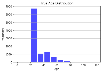
Firstly, we plot the original distribution of the Age column.

import matplotlib.pyplot as plt
import numpy as np
%matplotlib inline

ages = list(range(0, 130, 10))
age = df_diabetes.Age

# Plot a histogram with 10-year bins
n_age, bins, patches = plt.hist(age, bins=ages, color='blue', alpha=0.7, rwidth=0.85)
plt.grid(axis='y', alpha=0.75)
plt.xlabel('Age')
plt.ylabel('Frequency')
plt.title('True Age Distribution')
plt.show()
print(n_age.astype(int))

import matplotlib.pyplot as plt

with sn.Analysis() as analysis:
     data = sn.Dataset(path = file_path, column_names = lst_cols)

     age_histogram = sn.dp_histogram(
             sn.to_int(data['Age'], lower=0, upper=120),
             edges = ages,
             upper = 10000,
             null_value = -1,
             privacy_usage = {'epsilon': 0.5}
           )

analysis.release()

plt.ylim([0,7000])
width=4
agecat_left = [x + width for x in ages]
agecat_right = [x + 2*width for x in ages]
plt.bar(list(range(0,120,10)), n_age, width=width, color='blue', alpha=0.7, label='True')
plt.bar(agecat_left, age_histogram.value, width=width, color='orange', alpha=0.7, label='Private')
plt.legend()
plt.title('Histogram of Age')
plt.xlabel('Age')
plt.ylabel('Frequency')
plt.show()

print(age_histogram.value)

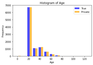
This visual shows that the true distribution of the Age column is like differentially private distribution. Hence, we can keep the statistical value of the data while adding some noise to the original data.

Conclusion

Finally, let me be explicit that this is an active area of research. Hence, it will keep evolving and is an exciting space as AI applications get mainstream. Finally, this article is for information. Therefore, we do not claim any guarantees regarding the same.