Machine Learning Interpretability for Isolation forest using SHAP

In our previous article, we covered Machine Learning interpretability with LIME and SHAP. We introduced the concept of global and local interpretability. Moreover, we demonstrated the use of LIME and SHAP.

However, as an example, we interpreted a classic supervised learning technique viz. Regression. We did not interpret any unsupervised Machine Learning techniques like Clustering, Anomaly Detection, etc. Hence, in this article, we will cover Isolation forest, an Anomaly Detection technique. Why do we choose Isolation Forest? Because it’s from the tree-based model family, which are hard to interpret, be it a supervised setting or an unsupervised one. This will be a natural transition from the previous article where we interpreted a supervised model viz. Regression.

Having said that, Unsupervised Learning, especially Anomaly Detection, is hard to tune, because of the absence of ground truth. Hence, Machine Learning Interpretability gives you an insight into how the algorithm is working. But, before that, let’s have some intuition about the Isolation Forest.

Intuition to Isolation Forest.

Isolation forest is a tree-based Anomaly detection technique. What makes it different from other algorithms is the fact that it looks for “Outliers” in the data as opposed to “Normal” points. Let’s take a two-dimensional space with the following points:

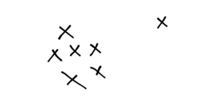
We can see that the point at the extreme right is an outlier. The intuition behind the Isolation Forest is that outliers can be separated with smaller tree depths. Now, we know that tree-based methods tessellate the space into rectangles. Every line that breaks the space is a node in a decision tree. Let’s take an example. We tessellate the space and observe the number of tessellations needed to isolate the outlier:

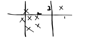
Drawing lines randomly in order, we need 3 lines to separate the outlier. Let’s take another case:

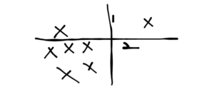
Here, you need only 2 lines to isolate the outlier. Now, let’s take the opposite case.

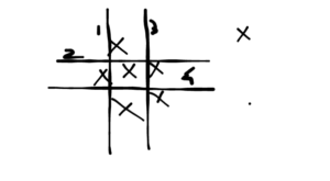
Let’s say we want to isolate the point right in the middle. It’s can be seen that 4 lines are needed to do so. This gives us an intuition of how Isolation Forest works. The mathematics of this technique is beyond this article. For that, the reader may go through the original research paper here.

Having said that, let’s go through some code using Sensor Data from Kaggle.

Step 1: Read the Data

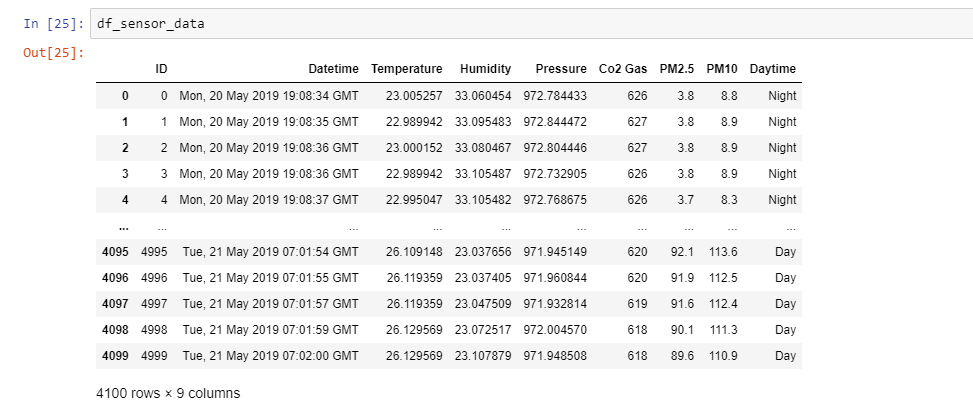
Download the sensor data from the above link and read it using Pandas:

import lime
import shap
import pandas as pd
import numpy as np
import matplotlib.pyplot as plt

df_sensor_data = pd.read_csv("./SensorData.csv")

Step 2: Prepare the Data and Describe it

In this step, we separate the numerical values from  ID, Datetime, and Daytime. Furthermore, we describe the data using pandas describe.

y = df_sensor_data[['ID','Datetime','Daytime']].values
X = df_sensor_data.drop(['ID','Datetime','Daytime'],axis = 1)

X.describe()

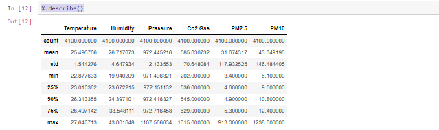
This gives us some idea about the distribution of every variable that matters. In all the variables, there is a spike from 75th to 100th percentile. However, for a better judgment of the distribution, let’s zoom into data above the 75th percentile.

percentiles = np.linspace(0.76, 1, num=25, endpoint=True) #To generate an array of percentiles from 76(0.76) to 100(1.0)
X.quantile(percentiles)

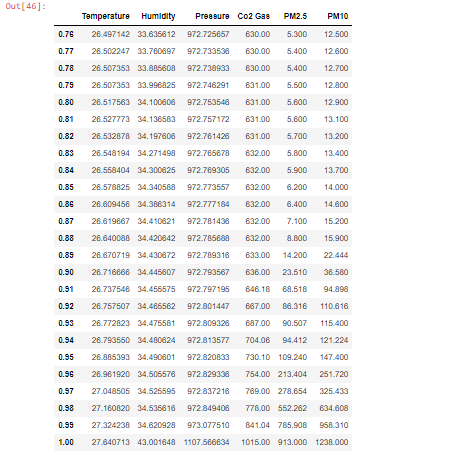
This gives us an idea of the number of outliers that may exist in the data. From the looks of it, we can see that the columns PM2.5 and PM10 (Air Quality Index) have a significant number of outliers. A simple google search will reveal that PM2.5 > 150 is harmful, while PM10>80 is serious. Hence, approximately 15 percent of values are outlier candidates. This sets us for using an Anomaly Detection algorithm like Isolation forest.

Step 3: Train an Isolation Forest model

In this step, we train an Isolation Forest with the default parameters:

from sklearn.ensemble import IsolationForest
iforest = IsolationForest(max_samples='auto',bootstrap=False, n_jobs=-1, random_state=42)

iforest_= iforest.fit(X)

y_pred = iforest_.predict(X)

Further, we calculate the Anomaly Score using the decision_function() method of iforest. A positive score shows a normal point, whereas a negative score represents an Anomalous point.

y_score = iforest.decision_function(X)

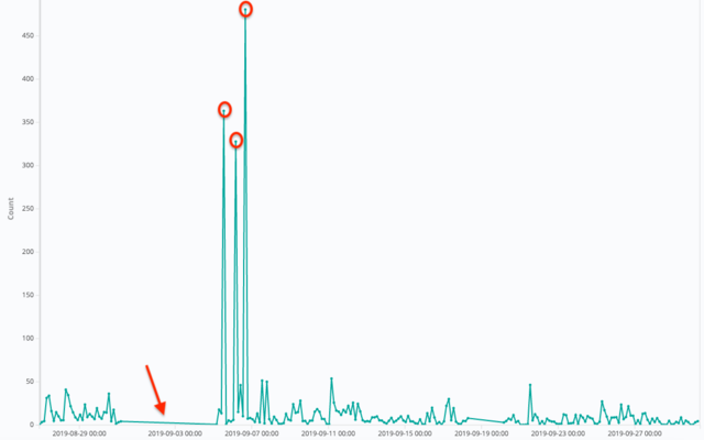
From the scores, we can find the points that have been predicted/marked as anomalous:

neg_value_indices = np.where(y_score<0)
len(neg_value_indices[0])

The length of the array is 574. That means there are 574 anomalous points, which is 14 percent of 4100. This is in line with our estimate that around 15 per cent of data points could be anomalous.

Step 4: Machine Learning Interpretability

From the previous article on Machine Learning Interpretability, we know SHAP can give global and local interpretability. Moreover, we saw SHAP has a specialized explainer for Tree-based models viz. TreeExplainer. Since Isolation Forest is tree-based, let’s follow similar steps here:

A Tree Explainer

First, create an explainer object and use that to calculate SHAP values.

exp = shap.TreeExplainer(iforest) #Explainer
shap_values = exp.shap_values(X)  #Calculate SHAP values
shap.initjs()

Global Machine Learning Interpretability

The next step is creating a summary plot. Summary plots help us visualize the global importance of features.

shap.summary_plot(shap_values, X)

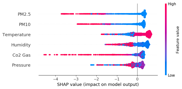
This plot gives us the impact of a particular variable on anomaly detection. Let’s take Co2 as an example. The summary plot says that high values of  Co2 show anomalous items while lower values are normal items.

A more comprehensive way to visualize the summary plot is as a bar plot.

shap.summary_plot(shap_values, X,plot_type="bar")

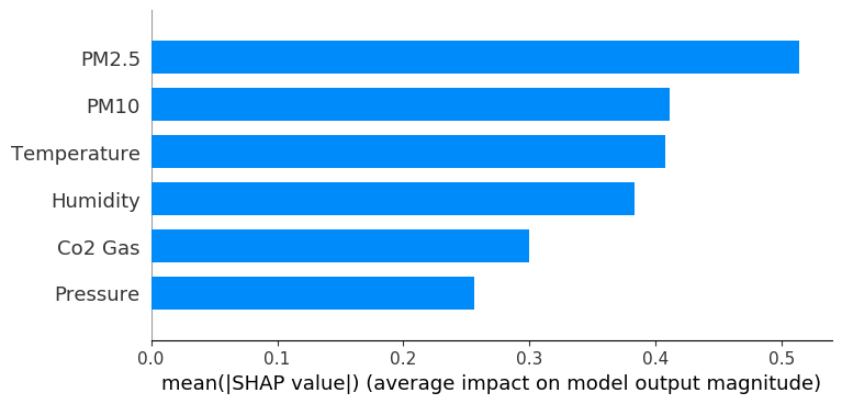
Evidently, the variables PM2.5 and PM10 have the highest average SHAP value. Hence, they have the highest impact on determining the anomaly score. This corroborates our observations while exploring the descriptive statistics of the data.

Having said that, let’s explain the predictions for a single instance.

Local Machine Learning Interpretability

The beauty of local interpretability is that it gives explanations for a particular point, which may differ from global explanations. Let’s take an example. One of the indices in neg_value_indices, i.e. the indices of anomalous points, was found to be 1041. Let’s explain this instance using a force plot and a bar plot.

A force plot is a visual that shows the influence of feature(s) on the predictions.

shap.force_plot(exp.expected_value, shap_values[1041],features =X.iloc[1041,:] ,feature_names =X.columns)

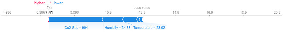
In this example,  Co2 and Humidity are pushing the outcome towards being an anomaly. Again, a better way to see local explanations is a bar plot.

shap.bar_plot(shap_values[1041],features =X.iloc[1041,:] ,feature_names =X.columns )

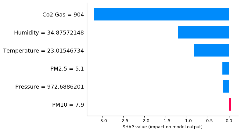
It is clear from the above plot that high Co2 and Humidity show anomalous behaviour. Moreover, PM2.5 and PM10 are not out of bound. Hence, this point does not follow the global trend where the two aforementioned variables are primary determinants of anomaly.

Conclusion

We hope this article on Machine Learning Interpretability for Isolation Forest is useful and intuitive. Please note that this is for information only. We do not claim any guarantees regarding the code, data, and results. Neither do we claim any guarantees regarding its accuracy or completeness.

Featured Image Credit: Wikipedia