Explainable Machine Learning with Azure Machine Learning

In the previous two articles, we took a dive into Explainable Machine Learning. The first one dealt with LIME and SHAP for a supervised machine learning setting. The second one dealt with an unsupervised use case viz. Anomaly Detection using Isolation Forest. We explained the same using SHAP.

You may note that we used open-source libraries like LIME and SHAP to do so. However, with advancements in cloud technologies, various other tools and libraries are making headway. In Microsoft Azure, the library for Interpretable Machine Learning is azureml-interpret. In this article, we will use this library to perform Interpretable ML.

Explainable Machine Learning with azureml-interpret

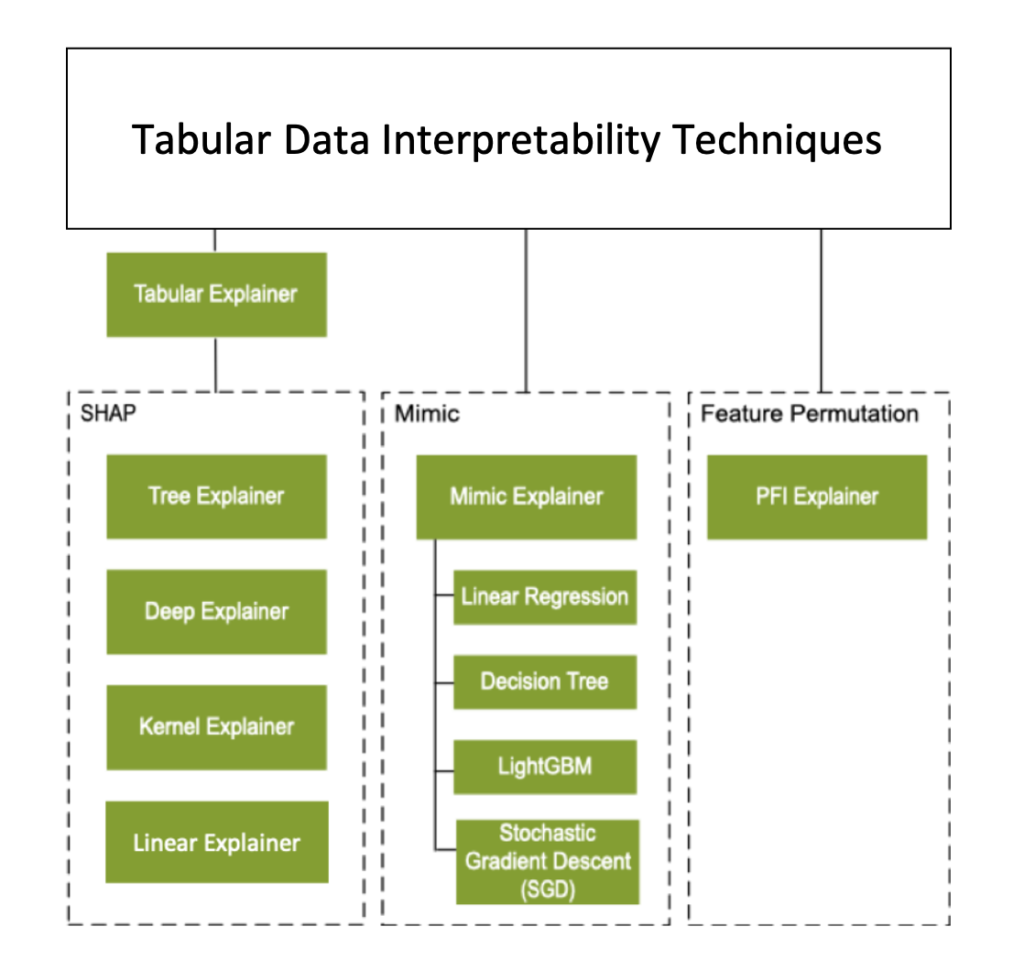
The azureml-interpret package has the following explainers:

• MimicExplainer: This explainer creates a global surrogate model that approximates your trained model, which explains your model. The surrogate model architecture should be the same as the trained model.
• TabularExplainer: This one acts as a wrapper around various SHAP algorithms. It selects the explainer based on the model to be explained.
• PFIExplainer: This is the classic Permutation Feature Importance explainer, which shuffles feature values to measure the impact on predictions. Please note that this technique can provide Global Explanations only.

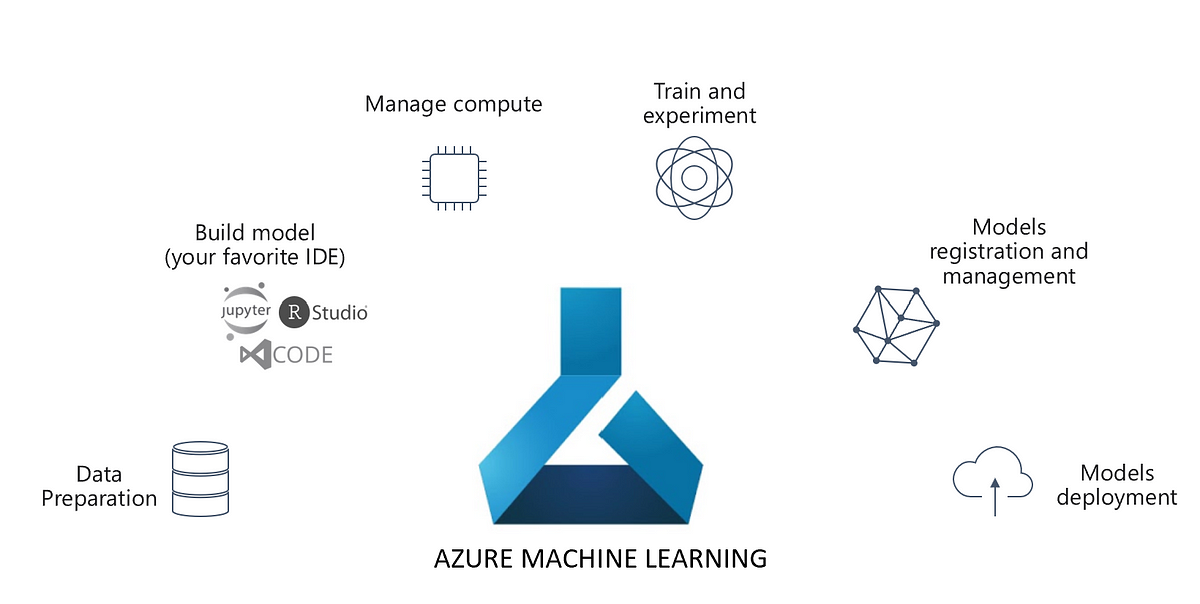
In summary, here is a diagram from Microsoft:

Furthermore, let’s go through hands-on code. Similar to our article on LIME and SHAP, we will use the California Housing Dataset. For details, we strongly recommend you to read our first article in the beginning. Besides, we will learn some concepts of Azure Machine Learning like Experiments, Environments, etc. However, we will use only the TabularExplainer. You can try the other explainers for yourself.

But before moving further, a question may arise what advantage does Azure Machine Learning brings in with all the aforementioned concepts?  The simple answer is logging and traceability. In a simple ML code, explainability is followed by training. In Azure ML, you can additionally log the explanations using an object called ExplanationClient. Now, let’s dive into the code.

Check the libraries

Got to Azure Machine Learning studio > Compute > Your Compute > Jupyter > Notebook and run the following command to verify if the requisite packages are installed:

!pip show azureml-explain-model azureml-interpret

Connect to Azure ML Workspace

Next, let’s connect to the Azure ML workspace from the notebook using the following script:

import azureml.core
from azureml.core import Workspace

# Load the workspace from the saved config file
ws = Workspace.from_config()

Create a training and explanation script

We will use the same model training script as used in the LIME and SHAP article with certain additions called Experiments. Let’s introduce the concept of Experiments in Machine Learning:

An experiment encapsulates any part of the Data Science life cycle, like EDA, Model Training, Deployment, etc. It’s a named process in Azure Machine Learning. An experiment can be performed multiple times. Each iteration of the experiment is called a run, which is logged under the same experiment.

In Azure ML, an experiment can be run in two ways viz. Inline and via ScriptRunConfig. 

Inline Experiments

As the name suggests, Inline experiments are created and run within the script to be executed. These experiments are good to perform rapid exploration and prototyping. We will understand generating explanations using an Inline Experiment. An example goes here:

from azureml.core import Experiment
import pandas as pd
import matplotlib.pyplot as plt
import numpy as np
import joblib
from sklearn.model_selection import train_test_split
from sklearn.datasets import fetch_california_housing
from xgboost import XGBRegressor
from sklearn.metrics import r2_score

# Import Azure ML run library
from azureml.core.run import Run

# Import libraries for model explanation
from azureml.interpret import ExplanationClient
from interpret.ext.blackbox import TabularExplainer
%matplotlib inline

# Create an Azure ML experiment in your workspace
experiment = Experiment(workspace=ws, name="california-housing-explain")

# Start logging data from the experiment, getting a reference to the experiment run
run = experiment.start_logging()
print("Starting experiment:", experiment.name)

#The script to be run starts here

# load the dataset
california_housing = fetch_california_housing()
pd_df_california_housing = pd.DataFrame(california_housing.data, columns = california_housing.feature_names)
pd_df_california_housing['target'] = pd.Series(california_housing.target)


# Separate features and labels target
features = california_housing.feature_names
labels = california_housing.target
X, y = pd_df_california_housing[features].values, pd_df_california_housing['target'].values

# Split data into training set and test set
X_train, X_test, y_train, y_test = train_test_split(X, y, test_size=0.30, random_state=0)

# Train a XgBoost model
print('Training a XgBoost model')
xgb = XGBRegressor(n_estimators=200, max_depth=5) 
xgb.fit(X_train, y_train)


# calculate R2 Score
y_pred = xgb.predict(X_test)
r2_score = test_r2_score = r2_score(y_test, y_pred)
print('R2 Score: ' + str(r2_score))

print('Model trained.')

os.makedirs('outputs', exist_ok=True)
# note file saved in the outputs folder is automatically uploaded into an experiment record
joblib.dump(value=xgb, filename='outputs/california_housing.pkl')

#Model Explainability

# Get an explanation
explainer = TabularExplainer(xgb, X_train, features=california_housing.feature_names)   
explanation = explainer.explain_global(X_test)

# Get an Explanation Client and upload the explanation
explain_client = ExplanationClient.from_run(run)                 
explain_client.upload_model_explanation(explanation, comment='Tabular_Explanation')

#The script to be run ends here

#Complete the run
run.complete()

Let’s review the high-level steps here:

1. Import Libraries
2. Create an Experiment
3. Start the Run
4. Train the Model and save it
5. Generate and Upload Explanations
6. Close the Experiment Run.

Note the section Model Explainability. It comprises two steps:

1. Creating an Explainer that generates Explanations.
2. Uploading the Explanations to the Experiment Run.

Having said that, this code will run on the Compute instance in which this script is authored. What if you want to run it on a different compute cluster? What if you wish to run this script with multiple parameters on different Compute Clusters? This code is neither scalable nor re-usable. ScriptRunConfig class addresses these challenges.

However, if you are not interested in ScriptRunConfig, navigate to the final section of this article i.e. Viewing Explanations in Azure ML.

ScriptRunConfig class

The ScriptRunConfig class takes many parameters. For more details, refer to this link. However, we will use the following parameters:

• source_directory: Directory in which the script is saved.
• script: The training and explanation script.
• compute_target: The compute target name.
• environment: The environment used.

Step 1: Creating source_directory

First, create a dedicated folder for the experiment i.e. source directory.

import os, shutil
from azureml.core import Experiment

# Create a folder for the experiment files
experiment_folder = 'california_train_and_explain'
os.makedirs(experiment_folder, exist_ok=True)

Step 2:  Defining script

Further, create the training script.

%%writefile $experiment_folder/california_training.py
# Import libraries
import pandas as pd
import numpy as np
import joblib
from sklearn.model_selection import train_test_split
from sklearn.datasets import fetch_california_housing
from xgboost import XGBRegressor
from sklearn.metrics import r2_score


# Import Azure ML run library
from azureml.core.run import Run

# Import libraries for model explanation
from azureml.interpret import ExplanationClient
from interpret.ext.blackbox import TabularExplainer

# Get the experiment run context
run = Run.get_context()

# load the dataset
california_housing = fetch_california_housing()
pd_df_california_housing = pd.DataFrame(california_housing.data, columns = california_housing.feature_names)
pd_df_california_housing['target'] = pd.Series(california_housing.target)


# Separate features and labels.
features = california_housing.feature_names
labels = california_housing.target
X, y = pd_df_california_housing[features].values, pd_df_california_housing['target'].values

# Split data into training set and test set
X_train, X_test, y_train, y_test = train_test_split(X, y, test_size=0.30, random_state=0)

# Train a XgBoost model
print('Training a XgBoost model')
xgb = XGBRegressor(n_estimators=200, max_depth=5) 
xgb.fit(X_train, y_train)


# calculate R2 Score
y_pred = xgb.predict(X_test)
r2_score = test_r2_score = r2_score(y_test, y_pred)
print('R2 Score: ' + str(r2_score))

print('Model trained.')

os.makedirs('outputs', exist_ok=True)
# note file saved in the outputs folder is automatically uploaded into experiment record
joblib.dump(value=xgb, filename='outputs/california_housing.pkl')

# Get an explanation
explainer = TabularExplainer(xgb, X_train, features=california_housing.feature_names)
explanation = explainer.explain_global(X_test)

# Get an Explanation Client and upload the explanation
explain_client = ExplanationClient.from_run(run)
explain_client.upload_model_explanation(explanation, comment='Tabular Explanation')

# Complete the run
run.complete()

This script writes a file california_training.py under the folder name california_train_and_explain. Please notice the difference in the bold section of the script. We haven’t created the experiment here. But, we get the run context. It is the current service context (environment, compute etc.) in which an experiment runs.

Step 3: Creating Compute Cluster

Furthermore, let’s define the compute. The following script creates a compute cluster if it doesn’t exist.

from azureml.core.compute import ComputeTarget, AmlCompute
from azureml.core.compute_target import ComputeTargetException

cluster_name = "int-cluster"

try:
    # Check for existing compute target
    interpret_cluster = ComputeTarget(workspace=ws, name=cluster_name)
    print('Found existing cluster, use it.')
except ComputeTargetException:
    # If it doesn't already exist, create it
    try:
        compute_config = AmlCompute.provisioning_configuration(vm_size='STANDARD_DS11_V2', max_nodes=2)
        interpret_cluster = ComputeTarget.create(ws, cluster_name, compute_config)
        interpret_cluster.wait_for_completion(show_output=True)
    except Exception as ex:
        print(ex)

Step 4: Creating environment file

Let’s create an environment file. An Environment is the settings in which a code runs. Hence, an environment file comprises the dependencies needed to run the code. This is a necessary step since the cluster created in the previous step may not have the packages installed. For instance, we are using XgBoost, which may not be available in the int-cluster.

Here is the environment file:

%%writefile $experiment_folder/interpret_env.yml
name: interpret_environment
dependencies:
- python=3.6.2
- scikit-learn
- xgboost
- pandas
- joblib
- pip
- pip:
  - azureml-defaults
  - azureml-interpret

During runtime, these packages are installed in a remote target environment.

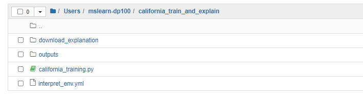
Step 5: Running the experiment using ScriptRunConfig

Finally, with all the parameters in place, let’s create an experiment to run Explainable Machine Learning using ScriptRunConfig. But before that, here is the folder structure that comprises the training script california_training and the interpret_env environment file.

from azureml.core import Experiment, ScriptRunConfig, Environment
from azureml.widgets import RunDetails


# Create a Python environment for the experiment
explain_env = Environment.from_conda_specification("explain_env", experiment_folder + "/interpret_env.yml")

# Create a script config
script_config = ScriptRunConfig(source_directory=experiment_folder,
script='california_training.py',
environment=explain_env,compute_target=interpret_cluster)

# submit the experiment
experiment_name = 'california-housing-explain'
experiment = Experiment(workspace=ws, name=experiment_name)

run = experiment.submit(config=script_config)

RunDetails(run).show()
run.wait_for_completion()

Viewing Explanations in Azure ML

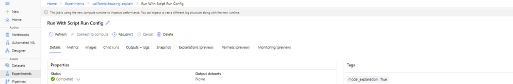
In the Azure ML Studio, go to the experiments section. Open the experiment california-housing-explain. Open the latest run and edit the Run name. The key difference between Inline and ScriptRunConfig experiments is the Compute Target and the Run Type as displayed below.

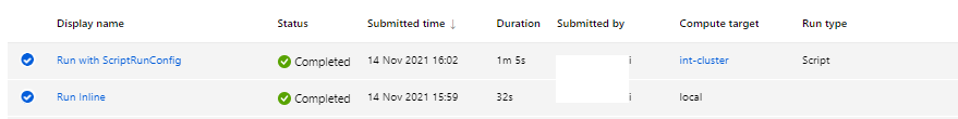
Alternatively, when you run with ScriptRunConfig, you can click on the View run details as shown in the previous image.

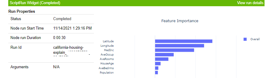
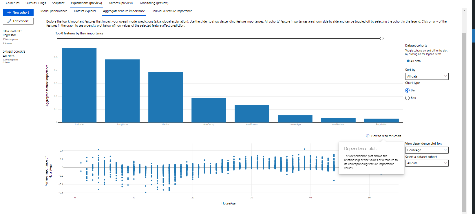
Global Explanations

To view ML Model explanations, navigate to the Explanations section. The first tab to appear is the Aggregate Feature Importance, which is the global feature importance. This is like a summary plot in SHAP.

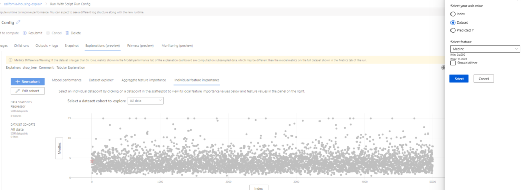
Local Explanations

Furthermore, switch to the individual feature Importance and click on the Y-Axis. Change it to Predicted Y.

Lastly, click on any random point and observe the feature importance for that point. Our random click took us to row number 2483

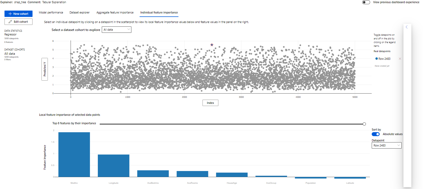
Evidently, the Median Income feature matters the most!

Conclusion

Hope this article helps. However, we don’t claim any guarantees about it. Reader discretion is advised.