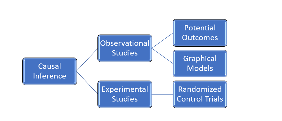
By nature, humans are inquisitive. We want to know the cause of everything that happens to us. In fact, the cause-effect phenomenon is central to Indian Philosophy in the form of Karma. This is truer in businesses, where root cause analysis plays a vital role. Hence, Causal Inference becomes key to Data Science and Analytics. But there are various ways in which you can infer causal relationships. Below are the main ways:
The gold standard of inferring Causal Relationships is Randomized Control Trials. However, we cannot perform experiments in every scenario due to the following considerations:
Ethics
Although we may want to perform Experimentation may be unethical in some cases. For instance, to know the effect of smoking on cancer, we cannot make people smoke. It’s outright unethical.
Feasibility
Moreover, some experiments may be infeasible to perform. For instance, it’s highly infeasible to divide countries into Capitalist or Communist regimes to measure their effect on GDP.
Possibility
Lastly, in several cases, it may be outright impossible to perform experiments. For instance, one’s DNA cannot be changed to see its effect on certain types of Cancer.
Hence, in a lot of real-world applications, it becomes imperative to learn causal relations from Observational data. Now, there are two major frameworks, using which Causal Relationships could be learnt.
Potential Outcomes Framework
The potential outcomes framework is a school of causality to infer the treatment effect of binary variables. It relies on a Statistical estimand to calculate a Causal quantity. Let’s try to understand this in more detail.
Let Y be the outcome and T be the treatment. In simpler terms, Y is the potential effect and T is the potential cause. Taking a medical example, Y could be headache and T could be the action of taking a pill. We would like to study if taking a pill reduces headache. To make things simple, if taking a pill reduces headache, we can assign the Treatment to be true or 1. Else, it is 0.
Now, if we want to calculate the effect of treatment on an individual, also called Individual Treatment effect, we can quantify it as follows:
Individual treatment effect (ITE): Yi(T=1) – Yi(T=0) :Yi(1) – Yi(0)
Here comes the fundamental problem of Causal Inference. If an individual is assigned T=1, we don’t have information about the effect when T=0. This is called the Counterfactual Scenario, which we cannot observe. To navigate this, we introduce Average Treatment Effect(ATE). The ATE is the average of Individual effects for the subset of population receiving the respective treatment:
Average treatment effect (ATE): E[Yi(1) – Yi(0)] = E[Y (1)] – E[Y (0)]
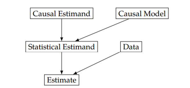
In the above ATE expression, the LHS i.e. E[Yi(1) – Yi(0)] is the Causal Estimand, whereas E[Y (1)] – E[Y (0)] is the statistical estimand, evaluated using data. Thus, the flow of getting an estimate using Potential Outcomes could be depicted as follows:

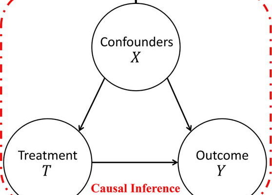
In real-world cases, we have confounders – variables that affect both treatment and outcomes. Hence, to find ATE of the treatment on the outcome, we need to adjust for the confounders. Suppose X is a confounder:
ATE with Adjustment: E[Y (1) – Y (0)] = EX E[ Y (1) – Y (0) | X] = EX [E[Y | T = 1, X] – E[Y | T = 0, X]]
Structural Causal Models
Another school of thought is the Structural Causal Models paradigm which is perhaps the most comprehensive framework in Causal Inference. It uses graphical models (Directed Acyclic Graphs, also called DAGs) to model the data-generating process, which is then tested against the available data. Moreover, it provides us with tools to model interventions, using the do operator, which is crucial to decision-making. Here is the flow of an SCM:
Having said that, SCM’s are largely based on a class of probabilistic graphical models called Bayesian Networks.
By now, you may have guessed that both the frameworks have similar flow. So, how is SCM related to Potential Outcomes? Let’s take a Causal Graph:
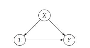
Here, Y is the Outcome, T is the treatment and X is the confounder. Here is the unifying expression:
E[Y| do(T=1)] – E[Y| do(T=0)] = EX [E[Y | T = 1, X] – E[Y | T = 0, X]]
The expression looks pretty similar to the Potential Outcomes expression above.
Conclusion
This is a brief introduction and overview of the two major frameworks of Causal Inference. To learn more about the same, read this excellent book by Neal Brady.
Also read, Mind over Data – Towards Causality in AI