Imagine that you receive a requirement to calculate the aggregations like average on a range of percentiles and quartiles, for a given dataset. There are two ways to approach this problem:
- Calculate actual percentile values and aggregate over the window.
- Fit a cumulative distribution and then aggregate over the window.
The first method has a normalizing effect over the data since it will interpolate values. To elaborate, let us take an example in excel.
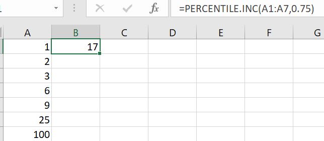
Here the cells A1: A7 is the dataset. Moreover, B1 is the 75th percentile which is not an actual value in the dataset. As mentioned earlier, this has a normalizing effect on the averages. We will understand this with the same example as above. Let us take a scenario where we want to have the average of top quantile values. Below are the values from 75th to 100th percentile for the same dataset.
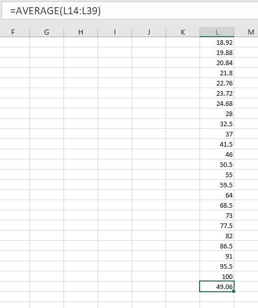
You can clearly see that the average of all the values from 75th to 100th percentile brings the average close to 49.06. However, if we consider the only two values from the top quantile present in the dataset, we get (100+25)/2 i.e. 62.5.
Now, one might be tempted to say that the first approach is better since it nullifies the effect of outliers like the value ‘100’. However, in industry, for appropriate assessment, one needs to consider the actual values rather than the interpolated values. Hence, here comes the concept of the Cumulative Distribution Function.
Also Read: Knowing when to consider Machine Learning
Cumulative Distribution Function
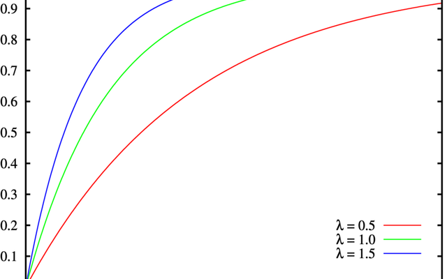
A cumulative distribution function for a continuous variable is the probability that the variable takes a value less than or equal to that value. For more on cumulative distribution, read this blog. However, it is important to note that the probability mentioned above is the ‘actual’ percentile value of the random value taken by the variable. To elaborate, if the CDF value is 0.8, 80 per cent of values in the dataset lie below that number.
Now, in case of the example mentioned above, if you want to calculate the average of all the values lying in the top quantile, all you need to do is fit a CDF and take values greater than or equal to 0.75. This is very much similar to TOP 25 per cent in SQL. However, the challenge here is that we need to do this on spark DataFrames. Here window functions come to our rescue.
Window Functions in Spark
Window functions help us perform certain calculations over a group of records called a ‘window’. These are also called as ‘over’ functions since they are built on lines of Over clause in SQL. Furthermore, they entail ranking, analytical and aggregate functions. For more details about window functions, refer to this document.
In this section, we will use the analytical function known as cume_dist() to fit a cumulative distribution on a dataset.
cume_dist for Cumulative Distribution
The cume_dist computes/fits the cumulative distribution of the records in the window partition, similar to SQL CUME_DIST(). The cume_dist assigns the percentile value to a number in the window/group under consideration. To demonstrate this, let us create spark dataframe similar to the data above in the excel.
Step 1: Create a Dataset
from pyspark.sql.functions import pandas_udf, PandasUDFType
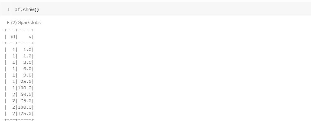
df = spark.createDataFrame(
[(1, 1.0),(1, 1.0), (1, 3.0), (1, 6.0), (1, 9.0),(1, 25.0),(1, 100.0),(2,50.0),(2,75.0),(2,100.0),(2,125.0)],
("id", "v"))
In this dataset, we have two columns id and v. The column ‘v’ consists of the values over which we need to fit a cumulative distribution. The id = 1 values consist of values similar to the excel example above. Moreover, we have 4 additional values with id = 2.
Step 2: Create a window
Next comes the important step of creating a window. The window creation consists of two parts viz. Partition By and Order By. Partition by helps us create groups based on columns, while order by specifies whether the analytical value should be based on ascending/descending order.
from pyspark.sql.window import Window

w = Window.partitionBy(df.id).orderBy(df.v)
In this case, we are partitioning by the column id, while the column ‘v’ is in ascending order(default). Hence, the percentile values will be based on the ascending order.
Step 3: Calculating the CDF
After creating the window, use the window along with the cume_dist function to compute the cumulative distribution. Here is the code snippet that gives you the CDF of a group i.e. the percentile values of all the values ‘v’ in the window partitioned by the column ‘id’.
from pyspark.sql.functions import cume_dist

cdf=df.select(
"id", "v",
cume_dist().over(w).alias("percentile")
)
Let us display the results of the CDF.
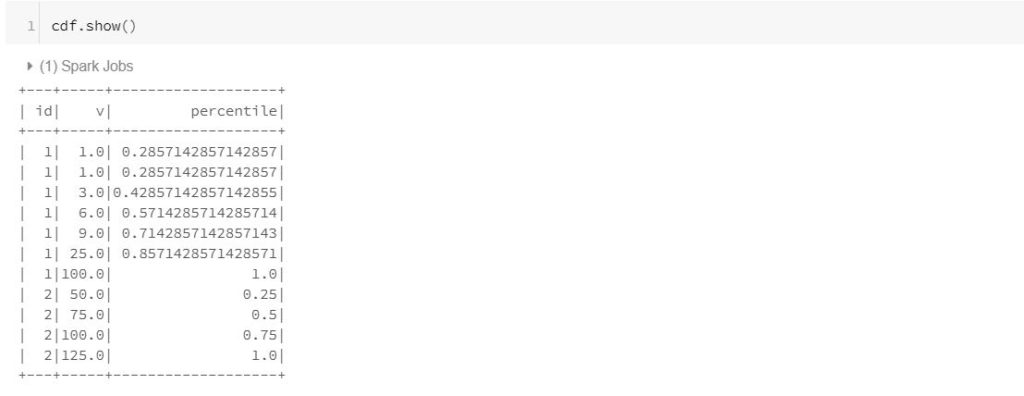
In the above results, it is evident that we have a percentile value corresponding to every value in the ‘v’ column.
Step 4: Top quantile average
Now, let’s go back to our original stated objective i.e. calculating the average of all the values above the 75th percentile. Hence, let us first filter out all the values above the 75th percentile.
cdf = cdf[cdf['percentile']>0.75]
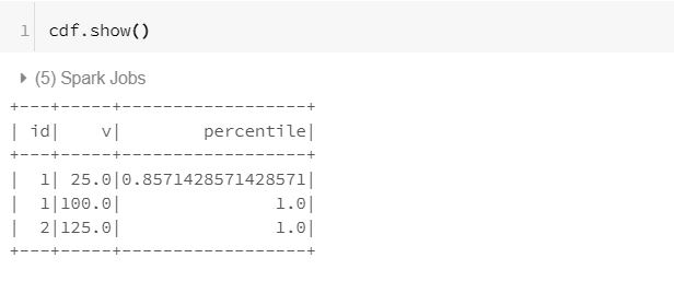
Finally, we calculate the average of top quantile with the below code snippet.
cdf.groupby('id').agg({'v':'avg'}).show()
The result is as follows:
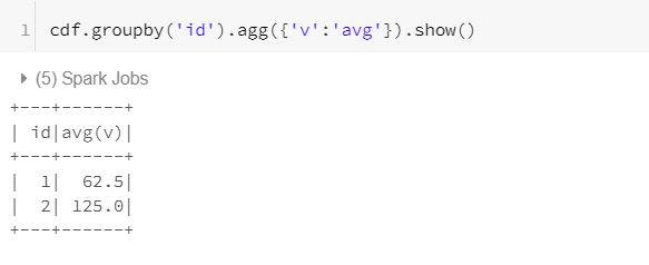
It is evident here that for id = 1, the top quantile average is (100+25)/2 i.e. 62.5. As expected!
Conclusion
We hope that you find this article useful. Please note that this is only for information purposes. We don’t claim it’s completeness. Kindly try it for yourself before adopting it.
Feature Image Credit: CC BY-SA 3.0, https://commons.wikimedia.org/w/index.php?curid=73794