Data Profiling options in Azure

The first step of Data Science, after Data Collection, is Exploratory Data Analysis(EDA). However, the first step within EDA is getting a high-level overview of how the data looks like. Some people may mistake it with Descriptive Statistics of Data. Descriptive statistics give us classic metrics like min, max, mean, etc. However, to know more about data, it won’t suffice. We need more information like metadata, relationships, etc. Here comes Data Profiling. To put it in different words, it is structure discovery, content discovery and relationship discovery of the data.

This brings us to the tools to perform profiling. We will start with Pandas Profiling and then later on move to profiling options in Azure Machine Learning and Azure Databricks.

Pandas Profiling

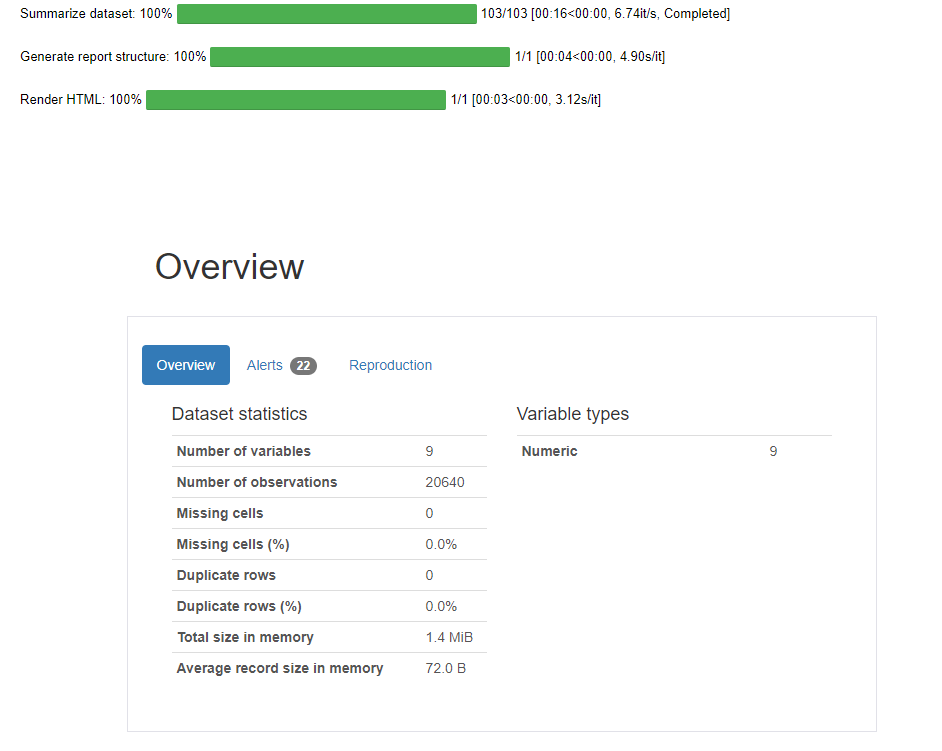
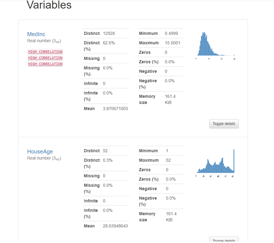
Our famous library pandas can perform data profiling. Let’s take our blog’s favourite dataset i.e. California Housing Dataset for profiling. This is a built in scikit learn dataset. We will first load it into a pandas dataframe and use the ProfileReport API of pandas_profiling library.

import pandas as pd
from sklearn.datasets import fetch_california_housing
from pandas_profiling import ProfileReport

california_housing = fetch_california_housing()

pd_df_california_housing = pd.DataFrame(california_housing.data, columns = california_housing.feature_names) 
pd_df_california_housing['target'] = pd.Series(california_housing.target)

profile = ProfileReport(pd_df_california_housing, title="Pandas Profiling Report", explorative=True)
profile

The object profile renders data profiling results as shown below.

Azure Machine Learning Dataset profiling

Pandas profiling is good for small datasets. But, with big data, cloud-scale options are necessary. Here come options like Azure Machine Learning. Azure Machine Learning provides the concept of datastores and datasets. Datastores are the linked services to the data stored in the cloud storage and datasets are the abstractions used to fetch data in Azure Machine Learning for Data Science. As a running example, let’s continue with the California housing dataset. We will perform the following steps:

• Upload California Housing to Azure Machine Learning workspace blob and create a dataset.
• Create an Azure Machine Learning Compute Cluster.
• Perform Data Profiling and view results.

Create the California Housing Dataset

For demonstration purposes, we will follow the below steps:

1. Load California housing dataset.
2. Load workspaceblobstore, the built-in datastore of Azure Machine Learning.
3. Upload the California housing dataset as a csv in workspaceblobstore.
4. Register a dataset using the csv.

But before that, let’s connect to the Azure ML workspace and create a folder for the Data Profiling experiment.

import azureml.core
from azureml.core import Workspace

# Load the workspace from the saved config file
ws = Workspace.from_config()
print('Ready to use Azure ML {} to work with {}'.format(azureml.core.VERSION, ws.name))

Folder creation:

import os
# Create a folder for the pipeline step files
experiment_folder = 'Data_Profiling'
os.makedirs(experiment_folder, exist_ok=True)

Furthermore, here is the script to create and register the dataset using the default workspaceblobstore:

import pandas as pd
from azureml.core import Dataset
from sklearn.datasets import fetch_california_housing

default_ds = ws.get_default_datastore()

if 'california dataset' not in ws.datasets:

# Register the tabular dataset
   try:
      california_housing = fetch_california_housing() 
      pd_df_california_housing = pd.DataFrame(california_housing.data, columns = california_housing.feature_names) 
      pd_df_california_housing['target'] = pd.Series(california_housing.target)

      local_path = experiment_folder+'/california.csv'
      pd_df_california_housing.to_csv(local_path)

      datastore = ws.get_default_datastore()

      # upload the local file from src_dir to the target_path in datastore
      datastore.upload(src_dir=experiment_folder, target_path=experiment_folder)

       california_data_set = Dataset.Tabular.from_delimited_files(datastore.path(experiment_folder+'/california.csv')) 

      try:
         california_data_set = california_data_set.register(workspace=ws, 
                                                            name='california dataset',
                                                            description='california data',
                                                            tags = {'format':'CSV'},
                                                            create_new_version=True)
         print('Dataset registered.')

      except Exception as ex:
         print(ex)

         print('Dataset registered.')

    except Exception as ex:
       print(ex)

else:
print('Dataset already registered.')

Create an Azure Machine Learning Compute Cluster

Here is the script to create or reuse the compute cluster:

from azureml.core.compute import ComputeTarget, AmlCompute
from azureml.core.compute_target import ComputeTargetException

cluster_name = "<your-cluster-name>"

try:
   # Check for existing compute target
   pipeline_cluster = ComputeTarget(workspace=ws, name=cluster_name)
   print('Found existing cluster, use it.')
except ComputeTargetException:
   # If it doesn't already exist, create it
  try:
    compute_config = AmlCompute.provisioning_configuration(vm_size='STANDARD_DS11_V2', max_nodes=2)
    pipeline_cluster = ComputeTarget.create(ws, cluster_name, compute_config)
    pipeline_cluster.wait_for_completion(show_output=True)
  except Exception as ex:
    print(ex)

Perform Data Profiling and view results

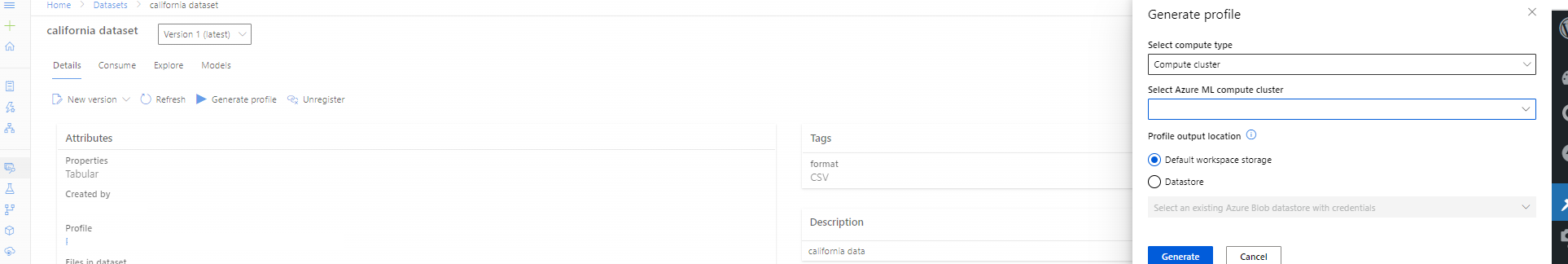
For Azure ML datasets, data profiling can be performed in two ways viz. using UI or using DatasetProfileRunConfig API. First, let’s take the UI route. In the Azure Machine Learning studio, go to Datasets > california dataset > Details > Generate Profile. Finally, select the compute of your choice.

This is a very simple way to perform data profiling in AML. However, mature organizations and teams would prefer an API to automate the same. In Azure ML, the DatasetProfileRunConfig will help you achieve the same. Here is the sample code:

from azureml.core import Experiment
from azureml.data.dataset_profile_run_config import DatasetProfileRunConfig

cal_dataset = Dataset.get_by_name(ws, name='california dataset')
DsProfileRunConfig = DatasetProfileRunConfig(dataset=cal_dataset, compute_target=<your-cluster-name>)
exp = Experiment(ws, "profile_california_dataset")
profile_run = exp.submit(DsProfileRunConfig)
profile_run.run.wait_for_completion(raise_on_error=True, wait_post_processing=True)
profile = profile_run.get_profile()

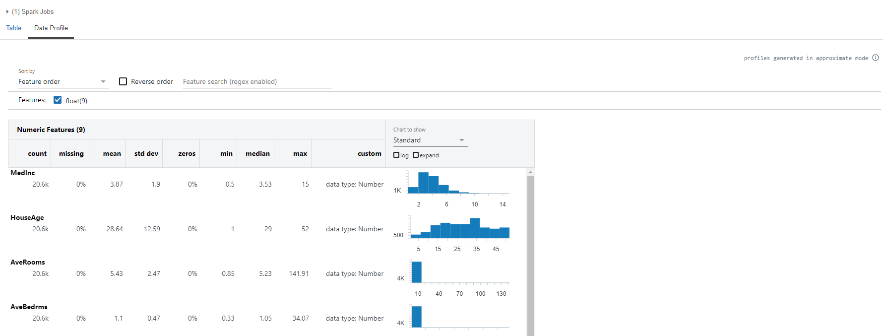
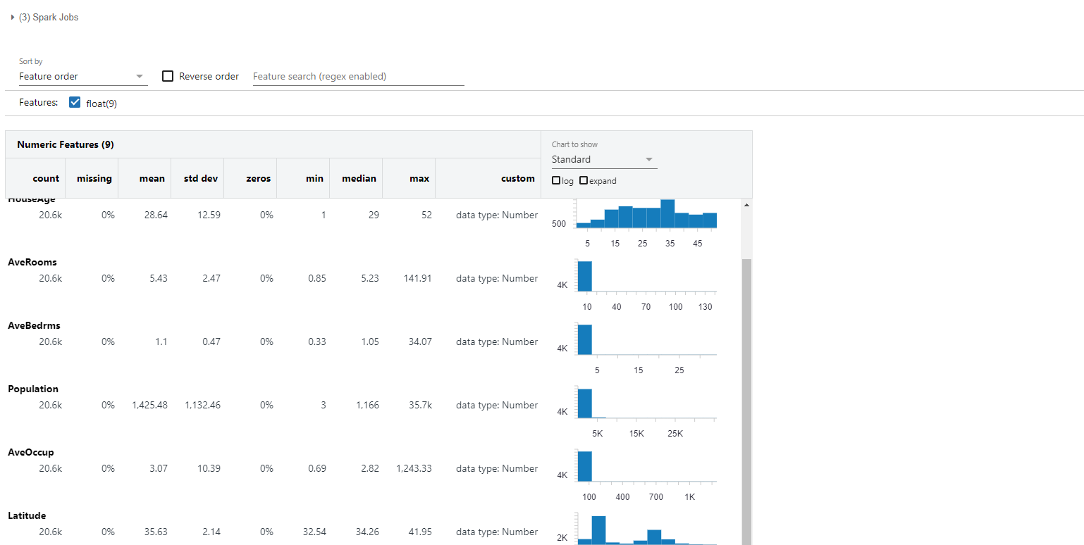
To view profiling results, go to Datasets > california dataset > Explore > Profile.

Azure Databricks profiling

Azure Databricks is one of the prominent PaaS offerings on Azure. Besides, it is a powerful Data Science Ecosystem like Azure Machine Learning. Hence, let’s look into the Data Profiling option in Azure Databricks. Please note that you need to provision a Databricks cluster with the runtime version above 9.1 to perform data profiling. Nonetheless, let’s lay out the steps to perform data profiling using Databricks.

Firstly, we load California Housing Dataset in a Pandas Dataframe

import pandas as pd 
from sklearn.datasets import fetch_california_housing

california_housing = fetch_california_housing()
pd_df_california_housing = pd.DataFrame(california_housing.data, columns = california_housing.feature_names) 
pd_df_california_housing['target'] = pd.Series(california_housing.target)

Secondly, we convert the Pandas Dataframe to Spark Dataframe and write it to Databricks Database as a table.

spark_df_california_housing = spark.createDataFrame(pd_df_california_housing)
spark_df_california_housing.write.mode("overwrite").saveAsTable("tbl_california_housing") #Optional Step

Lastly, we profile the dataframe using the display and/or dbutils API. The display command is databricks specific command, as opposed to the Spark show command. Nonetheless, the display gives you an option to get the data profiling as shown below:

display(spark_df_california_housing)

Apart from the display command, you can use the dbutils API to generate the data profiling from a Spark Dataframe. Databricks Utilities (dbutils) is a databricks library, used for many tasks pertaining to file systems, notebooks, secrets, etc. In our case, we will focus on dbutils.data utility, to understand and interpret datasets. Under dbutils.data, the summarize command renders the data profiling of a dataframe. It takes two parameters viz. the dataframe and precise. The latter, when set to True, gives the most accurate statistics of the data. Now, let’s perform the profiling.

dbutils.data.summarize(spark_df_california_housing, precise =True)

Notice that there is no tooltip saying profiles generated in the precise mode in this case, as opposed to the one with display function.

Conclusion

We hope this article is useful. Please note that this is for information. We do not claim any guarantees regarding its accuracy or completeness.