Introduction to Log Loss
Whenever we talk about performance metrics of the classification Machine Learning algorithms, the following names come to our mind:
- Accuracy
- Precision
- Recall
- F1-Score
- AUC
- Specificity
- Log Loss
Accuracy is the most intuitive metric. It is a percentage of correct predictions from the test/validation dataset. To understand Precision, Recall and F1 Score, we recommend you to read this article: Understanding Precision and Recall. AUC also called Area under the curve. It is the area under the curve formed by True Positive Rate vs False Positive Rate. Lastly, Specificity is the True Negative Rate. We won’t delve into much detail since these metrics are covered in great detail elsewhere.
Our metric for the day is Log Loss. Before going any further, let’s define it:
We will use the binary classification example. For a datapoint Xi ϵ Rd , yi ϵ {0,1} is the true label, while yi_pred represents the predicted probability. The log loss for this datapoint can be defined:
Log Loss (Xi , yi) = – yi * log(yi_pred ) ; yi = 1
= – (1 – yi ) * log(1 – yi_pred ) ; yi = 0
For the N points in a dataset, the average log loss can be defined as:
Log Loss (X , y) = -1/N * ΣiN=1 [yi * log(yi_pred) + (1 – yi ) * log(1 – yi_pred)]
Intuition to Log Loss
After defining log loss, let’s try to have an intuition. Machine Learning Classification algorithms can output probability of an instance belonging to a class, either inherently or by using calibration. Let’s say we consider the class ‘1’. So, how can we evaluate the predicted probabilities?
Here is the graph of negative log function (-log(x)):
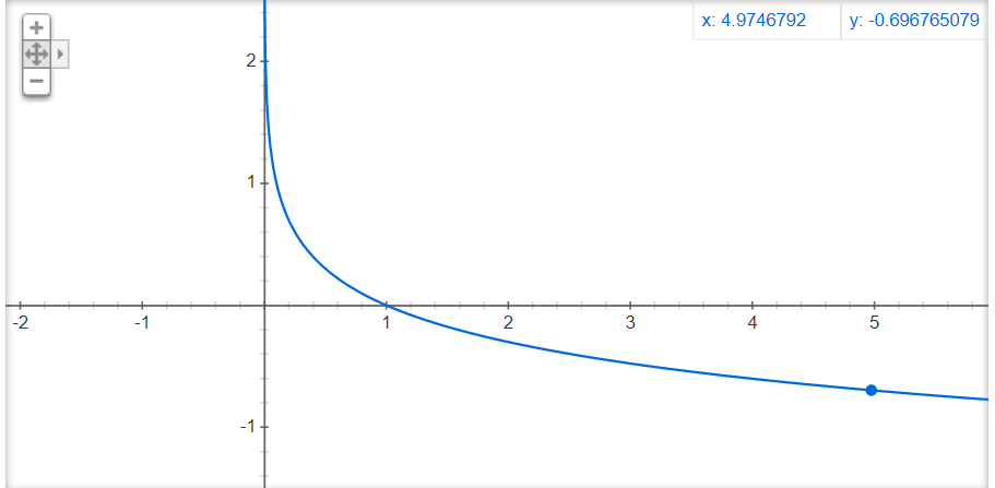
As we can see, lower the value of the x axis, bigger the value of -log (x). This negative log value is the penalty applied to the model for being far away from reality. Having said that, let’s look at how log loss function behaves using different cases. Here yi_pred = Pr(y =1)
Case 1: yi = 0 and yi_pred = 0.05
Log Loss = (1 – yi ) * – log(1 – yi_pred ).
= (1-0) * ( – log(1-0.05))
= 0.022
Interpretation: Since the actual class is 0 and the predicted probability is small (0.05), the negative log(1-yi_pred) is small i.e. 0.022. That means the penalty is small for being closer to reality.
Case 2: yi = 0 and yi_pred = 0.90
Log Loss = (1 – yi ) * – log(1 – yi_pred ).
= (1-0) * (- log(1-0.9))
= 1
Interpretation: Since the actual class is 0 and the predicted probability is big(0.90), the negative log(1-yi_pred) tends higher i.e. 1. That means the penalty is big for being far from reality.
Case 3: yi = 1 and yi_pred = 0.05
Log Loss = yi * – log(yi_pred ).
= 1* (- log(0.05))
= 1
Interpretation: Since the actual class is 1 and the predicted probability is small (0.05), the negative log(yi_pred) tends higher i.e. 1. That means the penalty is very high for being far from reality.
Case 4: yi = 1 and yi_pred = 0.90
Log Loss = yi * – log(yi_pred ).
= 1* (- log(0.05))
= 0.022
Interpretation: Since the actual class is 1 and the predicted probability is big(0.90), the negative log(yi_pred) is small i.e. 0.022. That means the penalty is big, being closer to reality.
For simplicity, let’s tabulate:
| yi(True Label) | yi_pred(Predicted Probability for class =1 ) | 1-yi_pred | Log Loss | Penalty |
| 0 | 0.05 | 0.95 | (1 – yi ) * -log(1 – yi_pred ) = 0.022 | Low |
| 0 | 0.9 | 0.1 | (1 – yi ) * -log(1 – yi_pred )= 1 | High |
| 1 | 0.05 | 0.95 | yi * -log(yi_pred ) = 1 | High |
| 1 | 0.9 | 0.1 | yi * -log(yi_pred ) = 0.022 | Low |
Hyperparameter tuning using Log Loss
In Machine Learning, Hyper parameter tuning is the key step. We find the best possible parameters for every algorithm by optimizing an evaluation metric. Selection of this metric depends on the business scenario. If the business requires high accuracy, Accuracy is the metric. If the business cares about being precise about the positive class, precision is the metric.
However, if the business cares about the confidence of the model, Log Loss can be considered. A key difference is that while the earlier metrics are maximized, the latter needs to be minimized. Let’s see an example using the Breast Cancer Dataset:
We will import some libraries first:
import numpy as np
import matplotlib.pyplot as plt
from sklearn import datasets
from sklearn.metrics import log_loss
from sklearn.model_selection import GridSearchCV
from sklearn.linear_model import LogisticRegression
from sklearn.model_selection import train_test_split
Next, let’s load the dataset and split the dataset into train, test and cross validation sets:
X, y = datasets.load_breast_cancer(return_X_y=True)
X_train, X_test, y_train, y_test = train_test_split(X, y, test_size=0.30, random_state=0)
X_train, X_cv, y_train, y_cv = train_test_split(X_train, y_train, test_size=0.30, random_state=0)
We will use Logistic Regression for simplicity, since it can predict probabilities naturally using the function predict_proba. A key hyper-parameter in Logistic regression is the regularization. Hence, we define a range of Regularization parameter:
reg = [0.0001,0.001,0.01,0.1,1]
Furthermore, let’s train the Logistic Regression model for each regularization value and calculate log loss on the cross validation dataset:
log_loss_array = []
for r in reg:

    lr = LogisticRegression(C=1/r, solver="liblinear").fit(X_train, y_train)
    y_pred = lr.predict_proba(X_cv)
    log_loss_array.append(log_loss(y_cv,y_pred[:,1]))
Let’s plot the log_loss_array:
plt.plot(reg, log_loss_array)
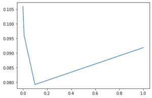
We can see that the loss is minimal for reg = 0.1. Hence, that is our Hyperparameter. Training the model on this value, we see the following results:
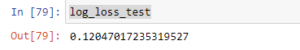
reg = 0.1
lr = LogisticRegression(C=1/reg, solver="liblinear").fit(X_train, y_train)
y_pred_test = lr.predict_proba(X_test)
log_loss_test = log_loss(y_test,y_pred_test[:,1])
log_loss_test
Advantages:
- We can gauge the confidence of the model’s prediction/performance.
Disadvantages
- It’s hard to interpret. Although the lowest value is 0, highest value can tend to infinity.
Conclusion
Finally, we hope this article is intuitive. We do not claim any guarantees regarding its accuracy or completeness.
Featured P.C. Wikipedia.