Before jumping to the Azure Databricks tutorial, it is good to know the evolution of the Data and AI space. Knowledge production started in ancient Sumerian civilization, with the advent of writing. However, it was bolstered with the silicon era. With Moore’s law, which says that the number of transistors in dense integrated circuit doubles about every two years, the cost of storage has reduced exponentially. As a result, we have witnessed an explosion of data in three dimensions viz volume, variety and velocity. A new era of big data ushered.
The evolution of Information systems
However, before we go to big data, it is imperative to understand the evolution of information systems. The journey commenced with extract files in the 1970s. Typically they were extracted from diverse sources residing in silos. Core banking systems were a typical instance of these kinds of systems. Non-standardization and conflicting information led to their downfall.
Later on, in the 1980s, distributed systems took precedence which used to fetch reports on the go directly from the source systems over the network. However, the technology of those times could not keep up to the increasing complexity of business requirements.
In the 1990s, the concept of data warehousing burst onto the canvas and revolutionized the landscape of Business Intelligence. Here data is extracted (E) from source systems, transformed online (T) and loaded into destination systems(L). The three steps combined formed ETL methodology
The Advent of Big Data
ETL jobs are scheduled in batches (typically 1-4 times a day). However, as businesses matured, information exploded in high volume, variety and velocity. Classic ETL tools could not handle such drastic change in the data landscape, e.g. ETL, tools and traditional databases could process structured data in batches, up to a specific volume. This gave birth to a new paradigm called big data. When big data was introduced, it brought in a plethora of tools and technologies; the most famous ecosystem being Hadoop, along with a shift in methodology from ETL to ELT. As discussed earlier, traditional ETL could not handle faster changes to data.
Also, memory and compute was an issue with traditional databases. This problem was solved with distributed file systems like HDFS and powerful compute like map reduce and spark. Though these ecosystems have significantly evolved, managing and leveraging them is a challenge, since there is a massive shortage of people who can handle all the aspects of these ecosystems. A classic implication of this predicament is the exclusivity of the toolset used data scientists and data engineers. This leads to a communication gap between the two teams with higher costs and increasing ETAs. This is the place where a unified analytics platform like Databricks comes into the picture.
Getting Started
Here is a comprehensive document on how to create an Azure Databricks workspace and get started. As the title suggests, Azure Databricks is a great platform for performing end to end analytics starting from batch processing to real-time analytics. Both batch processing and real-time pipelines form the lambda architecture.
I won’t reinvent the wheel in this article. Hence, for a detailed treatment of lambda architecture and batch processing refer to this article of mine: DataBricks – Big Data Lambda Architecture and Batch Processing
Also, here is another article elucidating on real-time analytics: DataBricks – Real-Time Analytics
It is important to remember that all the above data engineering effort is intended to enable analytics and more importantly predictive analytics. But before we dive into predictive analytics, it is important to understand the evolution of the broader paradigm of business analytics in general.
The evolution of Business Analytics
Firstly comes descriptive analytics. This approach is rooted in exploratory data analysis promoted by John Tukey. It is also called as traditional business intelligence and is closely related to data warehousing. It consists of compelling visuals and summary/analytical tables. More importantly, the central questions to perform this kind of analysis are ‘what happened?’ and ‘why did it happen?’ and it is mainly retrospective.
In due course, this manual analysis became impractical as datasets grew in dimensionality. As a result, data mining techniques were developed to find hidden insights in data leading to the trend of discovery analytics, which included techniques like Clustering, Associative rule mining etc.
However, a paradigm shift occurred when the approach shifted from ‘what happened’ and ‘why did it happen’ to ‘what might happen’. Thus the era of predictive analytics rose.
With anticipatory powers, human beings will gravitate towards taking corrective action. When predictions seem undesirable, a prescriptive analysis will be done and thus came in the term prescriptive analytics.
In this article, we will go through a detailed walkthrough on how to leverage databricks for machine learning.
Machine Learning with Azure databricks
As a part of this azure databricks tutorial, let’s use a dataset which contains financial data for predicting a probable defaulter in the near future. As a part of my article DataBricks – Big Data Lambda Architecture and Batch Processing, we are loading this data with some transformation in an Azure SQL Database. This how the data looks like:

This is a classification scenario in Machine Learning and the first column ‘SeriousDlqin2yrs’ is the label or the value to be predicted. In addition, here is the data dictionary of all the columns in the table:
| Variable Name | Description | Type |
| SeriousDlqin2yrs | A person experienced 90 days past due delinquency or worse | Y/N |
| RevolvingUtilizationOfUnsecuredLines | The total balance on credit cards and personal lines of credit except for real estate and no instalment debt like car loans divided by the sum of credit limits | percentage |
| age | Age of borrower in years | integer |
| NumberOfTime30-59DaysPastDueNotWorse | The number of times borrower has been 30-59 days past due but no worse in the last 2 years. | integer |
| DebtRatio | Monthly debt payments, alimony, living costs divided by monthly gross income | percentage |
| MonthlyIncome | Monthly income | real |
| NumberOfOpenCreditLinesAndLoans | Number of Open loans (instalment like car loan or mortgage) and Lines of credit (e.g. credit cards) | integer |
| NumberOfTimes90DaysLate | The number of times borrower has been 90 days or more past due. | integer |
| NumberRealEstateLoansOrLines | Number of mortgage and real estate loans including home equity lines of credit | integer |
| NumberOfTime60-89DaysPastDueNotWorse | The number of times borrower has been 60-89 days past due but no worse in the last 2 years. | integer |
| NumberOfDependents | Number of dependents in family excluding themselves (spouse, children etc.) | integer |
Azure Databricks Tutorial
Open an Azure Databricks Notebook as follows:
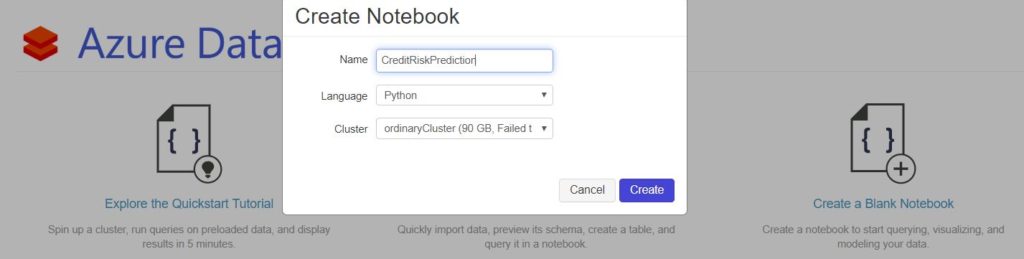
Notebook Creation
Importing libraries
Firstly, we start by importing important libraries in the first cell of the azure databricks notebook.
from pyspark.sql.types import *
from pyspark.sql.functions import *
from pyspark.sql.types import *
from pyspark.sql.functions import *

from pyspark.ml.classification import LogisticRegression
from pyspark.ml.feature import StringIndexer, VectorAssembler
from pyspark.ml.evaluation import BinaryClassificationEvaluator
Retrieving secrets
Next, we retrieve secrets from Azure key-vault . Secrets are a key vault feature for storing sensitive credential information. For Azure databricks, we achieve it using the key-vault backed secret scope. Here is the comprehensive documentation for setting up the same. In our case, we are storing login credentials for Azure SQL database. Further, we redact them using the following code:
jdbcUsername = dbutils.secrets.get(scope = "keyvaultsecrets", key = "username")
jdbcPassword = dbutils.secrets.get(scope = "keyvaultsecrets", key = "password")
Connection string
These retrieved credentials are used to create a JDBC connection string.
jdbcHostname = "newsignature.database.windows.net"
jdbcDatabase = "NewSignature"
jdbcPort = 1433
jdbcUrl = "jdbc:sqlserver://{0}:{1};database={2}".format(jdbcHostname, jdbcPort, jdbcDatabase)
connectionProperties = {
"user" : jdbcUsername,
"password" : jdbcPassword,
"driver" : "com.microsoft.sqlserver.jdbc.SQLServerDriver"
}
Importing and Exploring data
Once the connection is created, we connect to Azure SQL database and read the intended table.
pushdown_query = "(SELECT SeriousDlqin2yrs,cast(age as int) as age,cast([NumberOfTime30-59DaysPastDueNotWorse] as int) as NumberOfTime3059DaysPastDueNotWorse ,cast(DebtRatio as float) as DebtRatio,cast(NumberOfTimes90DaysLate as int) as NumberOfTimes90DaysLate,cast([NumberOfTime60-89DaysPastDueNotWorse] as int)as NumberOfTime6089DaysPastDueNotWorse from CreditData)cralias"
df = spark.read.jdbc(url=jdbcUrl,table=pushdown_query, properties=connectionProperties)
display(df)
Now as part of classification in Machine Learning, we need to identify the number of classes in the label.
df.groupby("SeriousDlqin2yrs").count().show()
Now, we are performing some elementary data cleansing tasks like removing duplicates and missing values using the following code snippet.
Identifying duplicates
total_count = df.count()
unique_count=df.dropDuplicates().count()
print (total_count-unique_count)
Removing missing values and duplicates
df.dropDuplicates().dropna().count()
CleansedData = df.dropDuplicates().dropna()
CleansedData.describe().show()
Removing outliers
An indispensable part of data cleansing is identifying and removing outliers since they can impact model performance in ways untold. This code retrieves rows with column values below a certain threshold value:
CleansedData1 = CleansedData.filter("NumberOfTime3059DaysPastDueNotWorse<5")
print(CleansedData1.count())
CleansedData2 = CleansedData1.filter("NumberOfTimes90DaysLate<5")
print(CleansedData2.count())
CleansedData3 = CleansedData2.filter("NumberOfTime6089DaysPastDueNotWorse<5")
print(CleansedData3.count())
CleansedData4 = CleansedData3.filter("DebtRatio<1")
print(CleansedData4.count())
Splitting data
As part of the machine learning process, we split the data into train and test sets:
splits = CleansedData4.randomSplit([0.7, 0.3])
train = splits[0]
test = splits[1]
train_rows = train.count()
test_rows = test.count()
print ("Training Rows:", train_rows, " Testing Rows:", test_rows)
Oversampling minority class
In the data exploration step, we found that this is a skewed dataset i.e. the negative class (label ‘0’) is much higher in count than positive class (label ‘1’). Hence, we perform oversampling in order to balance them.
from pyspark.sql.functions import rand

pos = train.filter("SeriousDlqin2yrs = 1")
neg = train.filter("SeriousDlqin2yrs = 0")

# undersample the most prevalent class to get a roughly even distribution
posCount = pos.count()
negCount = neg.count()

if posCount < negCount:
  pos = pos.sample(True, negCount/posCount)
else:
  neg = neg.sample(True, posCount/negCount)

# shuffle into random order (so a sample of the first 1000 has a mix of classes)
train = neg.union(pos).orderBy(rand())

#CleansedData4.createOrReplaceTempView("CreditCleansedData")

# Show the statistics
train.describe().show()
After resampling, we assign the train set to a new variable train_res.
train_res=train
train_res.groupby("SeriousDlqin2yrs").count().show()
In order to train the model using logistic regression, we need to have all the features in a single vector. We achieve it using VectorAssembler. Finally, we merge the assembled features with the label column to form the training set.
numericCols = ["age","NumberOfTime3059DaysPastDueNotWorse","DebtRatio","NumberOfTimes90DaysLate","NumberOfTime6089DaysPastDueNotWorse"]
assembler = VectorAssembler(inputCols=numericCols, outputCol="features")
training = assembler.transform(train_res).select(col("features"), col("SeriousDlqin2yrs").alias("label").cast(IntegerType()))
Now we are ready to train the logistic regression model using sci-kit learn.
lr = LogisticRegression(labelCol="label",featuresCol="features",maxIter=10,regParam=0.3)
model = lr.fit(training)
print ("Model trained!")
While testing the model, we include the label column as ‘trueLabel’, as it is the ground reality against which the model predictions will be tested.
testing = assembler.transform(test).select(col("features"),  col("SeriousDlqin2yrs").alias("trueLabel").cast(IntegerType()))
testing.show()
Now, we derive predictions from the model using the test set.
prediction = model.transform(testing)
predicted = prediction.select("features", "probability", col("prediction").cast("Int"), "trueLabel")
predicted.show(100, truncate=False)
Once the prediction is ready, we compute the model evaluation variables viz true positive, true negative, false positive and false negative.
tp = float(predicted.filter("prediction == 1.0 AND truelabel == 1").count())
fp = float(predicted.filter("prediction == 1.0 AND truelabel == 0").count())
tn = float(predicted.filter("prediction == 0.0 AND truelabel == 0").count())
fn = float(predicted.filter("prediction == 0.0 AND truelabel == 1").count())
metrics = spark.createDataFrame([
 ("TP", tp),
 ("FP", fp),
 ("TN", tn),
 ("FN", fn),
 ("Precision", tp / (tp + fp)),
 ("Recall", tp / (tp + fn))],["metric", "value"])
metrics.show()
Next, we go ahead to calculate the Area under curve (AUC).
prediction.select("rawPrediction", "probability", "prediction","trueLabel").show(100, truncate=False)
evaluator = BinaryClassificationEvaluator(labelCol="trueLabel", rawPredictionCol="rawPrediction", metricName="areaUnderROC")
auc = evaluator.evaluate(prediction)
print ("AUC = ", auc)
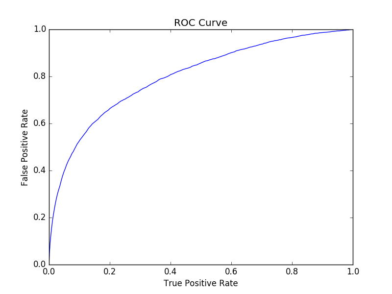
Finally, we plot the ROC curve using the famous matplotlib library of python.
import matplotlib.pyplot as plt
import numpy as np
trainingSummary = model.summary

#print(roc)
roc = trainingSummary.roc.toPandas()
plt.plot(roc['FPR'],roc['TPR'])
plt.ylabel('False Positive Rate')
plt.xlabel('True Positive Rate')
plt.title('ROC Curve')
plt.title('ROC Curve')
display(plt.show())
Conclusion
Hope you found this article informative. Stay tuned to data4v for more exciting posts in future.


Excellent article. Thanks for sharing your knowledge.