Tutorial: Hierarchical Clustering in Spark with Bisecting K-Means

In the previous article, we covered the standard K-Means Clustering technique on Spark. Read that article here: Tutorial : K-Means Clustering on Spark. In this article, we will walk through Hierarchical Clustering. It is a family of Clustering Algorithms that uses a hierarchical approach to divide the data into segments. It comes in two forms viz. Agglomerative Clustering and Divisive Clustering. However, we won’t get into the mathematical details of the same. Please read this article.

Having said that, in spark, both K means and Hierarchical Clustering are combined using a version of K-Means called as Bisecting K-Means. It is a divisive hierarchical clustering algorithm. Moreover, this isn’t a comparison article. For detailed comparison between K-Means and Bisecting K-Means, refer to this paper. Let’s delve into the code.

Step 1: Load Iris Dataset

Similar to K-Means tutorial, we will use the scikit-learn Iris dataset. Please note that this is for demonstration. In the real world, we will not use spark for tiny datasets like Iris.

import pandas as pd
from sklearn.datasets import load_iris
from pyspark.sql import SparkSession

df_iris = load_iris(as_frame=True)

Convert it to Pandas Dataframe. Again, this is only for demonstration.

pd_df_iris = pd.DataFrame(df_iris.data, columns = df_iris.feature_names)
pd_df_iris['target'] = pd.Series(df_iris.target)

Next, convert it to spark Dataframe and drop the ‘target’ column, since it is unsupervised learning.

spark_df_iris = spark.createDataFrame(pd_df_iris)
spark_df_iris = spark_df_iris.drop("target")

Step 2: Find the optimal number of clusters using the silhouette method.

Silhouette score is an evaluation metric for the clustering algorithms. It is a measure of similarity between a data point and the other points in a cluster. Read more about it here.

The higher the silhouette score, the better is the clustering. Now, even in Bisecting K means clustering algorithm, the number of clusters (k) is the hyper-parameter to be tuned. But, before that, let’s create a vector assembler and transform raw features into a single set of features.

from pyspark.ml.feature import VectorAssembler
assemble=VectorAssembler(inputCols=[
'sepal length (cm)',
'sepal width (cm)',
'petal length (cm)',
'petal width (cm)'],outputCol = 'iris_features')

assembled_data=assemble.transform(spark_df_iris)

Next, we will run the silhouette method. Please note that Bisecting K-means does not have the initMode argument, since Kmeans++ initialization is exclusive to K-means.

from pyspark.ml.clustering import BisectingKMeans
from pyspark.ml.evaluation import ClusteringEvaluator

silhouette_scores=[]
evaluator = ClusteringEvaluator(featuresCol='iris_features', \
metricName='silhouette')
for K in range(2,11):

    BKMeans_=BisectingKMeans(featuresCol='iris_features', k=K, minDivisibleClusterSize =1)

    BKMeans_fit=BKMeans_.fit(assembled_data)

    BKMeans_transform=BKMeans_fit.transform(assembled_data) 

    evaluation_score=evaluator.evaluate(BKMeans_transform)

    silhouette_scores.append(evaluation_score)

Next, plot the silhouette scores against the number of clusters.

import matplotlib.pyplot as plt
fig, ax = plt.subplots(1,1, figsize =(10,8))
ax.plot(range(2,11),silhouette_scores)
ax.set_xlabel('Number of Clusters')
ax.set_ylabel('Silhouette Score')

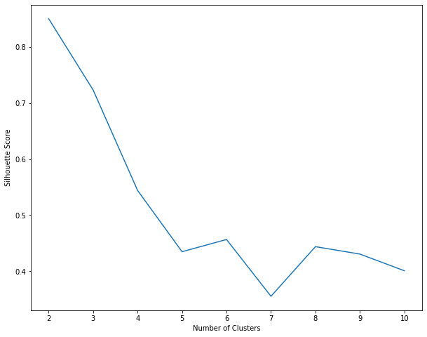
Similar to K Means, the local maximum is at K=3 i.e. 3 clusters will give us the best results (which is also the number of labels in the original dataset).

Step 3: Build the BisectingKMeans/Hierarchical Clustering model

Again, let’s build the model with 3 clusters.

BKMeans_=BisectingKMeans(featuresCol='iris_features', k=3) 
BKMeans_Model=BKMeans_.fit(assembled_data)
BKMeans_transform=BKMeans_Model.transform(assembled_data)

Step 4: Visualize Hierarchical Clustering using the PCA

Now, in order to visualize the 4-dimensional data into 2, we will use a dimensionality reduction technique viz. PCA. Spark has its own flavour of PCA.

First. perform the PCA. k=2 represents the number of principal components.

from pyspark.ml.feature import PCA as PCAml
pca = PCAml(k=2, inputCol="iris_features", outputCol="pca")
pca_model = pca.fit(assembled_data)
pca_transformed = pca_model.transform(assembled_data)

Next, extract the principal components

import numpy as np
X_pca = pca_transformed.rdd.map(lambda row: row.pca).collect()
X_pca = np.array(X_pca)

Next, retrieve the cluster assignments from bisecting k-means assignments.

cluster_assignment = np.array(BKMeans_transform.rdd.map(lambda row: row.prediction).collect()).reshape(-1,1)

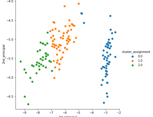
Finally, plot the principal components.

import seaborn as sns
import matplotlib.pyplot as plt

pca_data = np.hstack((X_pca,cluster_assignment))

pca_df = pd.DataFrame(data=pca_data, columns=("1st_principal", "2nd_principal","cluster_assignment"))
sns.FacetGrid(pca_df,hue="cluster_assignment", height=6).map(plt.scatter, '1st_principal', '2nd_principal' ).add_legend()
plt.show()

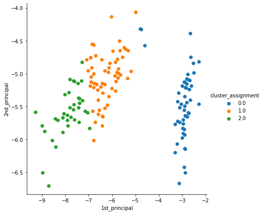
We urge you to read the previous article and observe the subtle difference between the clusters formed by both the algorithms (Hint Cluster 0.0 and 1.0).

Conclusion

We hope this article helps. This is only for information. We do not claim any guarantees regarding its completeness or accuracy.