Curve Fitting
Although Azure Machine Learning Studio is a great tool, it is basically a means to an end viz. Machine Learning. Before we dive into the new incarnation of this tool, let us spend some time contemplating Machine Learning in general.
Both physical and business worlds are replete with mathematical models in order to explain the various phenomenon. Let’s consider a very famous example of the Ohm’s law equation which goes as V= I*R. However, when we plot it experimentally, it looks like this:
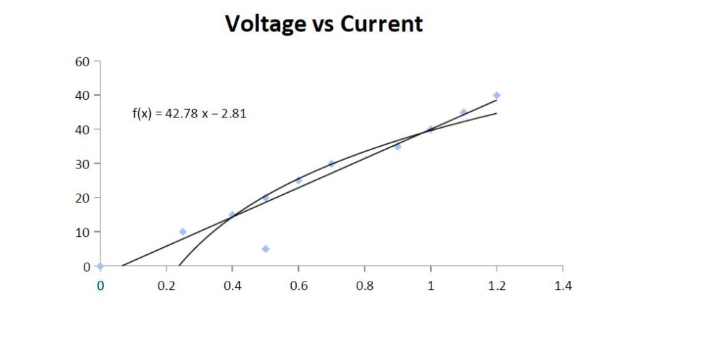
Even though the equation suggests a linear relationship between voltage and current, the experimental result deviates slightly i.e. all points do not lie on a straight line. We can explain this deviation with the fundamental definition of Ohm’s law which goes as follows:
So long as the physical conditions remain constant, the potential difference (voltage) across an ideal conductor is proportional to the current through it.
The key phrase in this definition is ‘physical conditions remain constant’. However, the real world is fraught with uncertainties, with fluctuating temperatures, humidity etc. Thus, we find the ‘best fit’ curve(line in this case) to verify an established phenomenon experimentally.
The Regression Line
In Ohm’s law, we have a well-defined mathematical model while curve fitting helps us verify the law experimentally. However, in practical business cases, instead of an established mathematical model, we have data received from various sources. Here, statistical techniques like regression come to our rescue. Along with curve fitting, regression uses the concept of correlation to figure out patterns/relations between two variables. For detailed, equations of regression and correlation, refer to this blog. Consider the below plot displaying Urea content in urine vs the osmotic pressure.

Here Urea in Urine is the dependent variable and Osmotic pressure is the independent variable. While correlation gives us the degree of dependence of urea on osmotic pressure, regression enables us to figure out the equation of the line passing through the points. Please note that correlation is not causation i.e. the independent variable does not necessarily cause the dependent variable.
Moving to Machine Learning
The above technique of curve fitting also called as Ordinary Least Squared technique works well with univariate data. However, as times passed, data grew in cardinality. Ordinary Least Squared technique became computationally expensive and made way for optimization techniques like gradient descent. These faster optimization techniques ushered in the era of Machine learning. Machine Learning can be classified into three major types as shown in the diagram below.
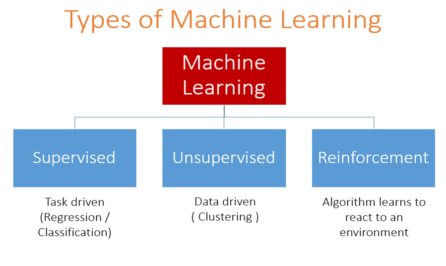
Source: Analytics Vidhya
In supervised learning, we have a dependent variable, which acts as ground truth to learn from. If the dependent variable is numerical, the task becomes regression, while if it is categorical, the task at hand is classification. Furthermore, if there is no ground truth to be learnt from, we have unsupervised techniques like clustering. Reinforcement learning is the paradigm which helps us learn from the environment.
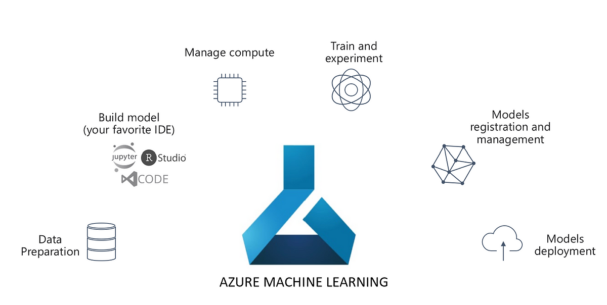
Azure Machine Learning Studio
As machine learning grew into prominence, the era of predictive analytics dawned. Businesses started leveraging the hidden patterns in data to predict outcomes based on historical trends, leading to the growth of Data Science. The rigorous mathematical discipline of Statistical modelling grew into a systematic business process. Data Science process entails data extraction, data preparation, modeling, training, testing and evaluation, deployment etc. Every phase requires an extensive amount of programming. However, not every organization intending to leverage the power of Data Science possesses the necessary skill set. To get a rough idea of the amount of programming required to build a simple classification model, read this article: Azure Databricks tutorial: an end to end analytics. To evade such an effort, drag and drop tools like Azure Machine Learning studio comes handy.
Data extraction
For this article, we will use credit card data to predict possible defaulters. The data lies in an Azure SQL Database table called CreditData. Here is the data dictionary:
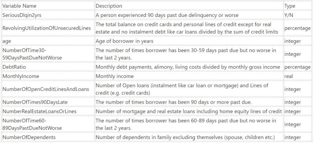
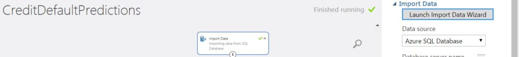
The first column i.e. SeriousDlqin2yrs is the label column (dependent variable), while the other columns are features (independent variable). Let us build a classification model to predict the same. Open the Azure Machine Learning studio and create a new experiment by clicking the New button at the bottom. In order to extract data from Azure SQL Database, we use the import module in AML studio. Click on the Launch Import Data Wizard and choose Azure SQL Database.
It contains the following fields:
- Database server name: The Azure SQL server which hosts your Azure SQL Database.
- Database name: The Azure SQL Database name.
- User name, Password: The SQL server user credentials.
- Query: The SQL query to extract data.
Data preparation
Once data is extracted from the SQL Database, we will use the module Apply SQL Transformation to remove missing values and outliers. You can write any SQL statement in this module. For instance, I will use the below query to do the same.
select * from t1 where (monthlyincome <> 'NA' OR NUMBEROFDEPENDENTS = 'NA') and ([NumberOfTime30-59DaysPastDueNotWorse]<5 and NumberOfTimes90DaysLate<5 and [NumberOfTime60-89DaysPastDueNotWorse]<5 and debtratio<5) ;
The table name t1 indicates that the data from the previous module is received on port 1 of the present module.
![]()
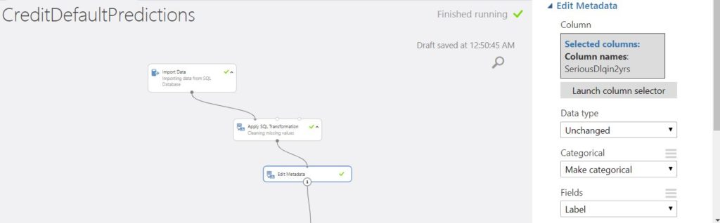
Further, since this is a classification problem, we use the Edit Metadata module to turn SeriousDlqin2yrs into a categorical variable and mark it as a label column as shown in the below image.
Modeling
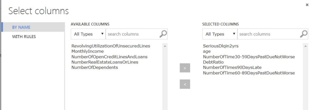
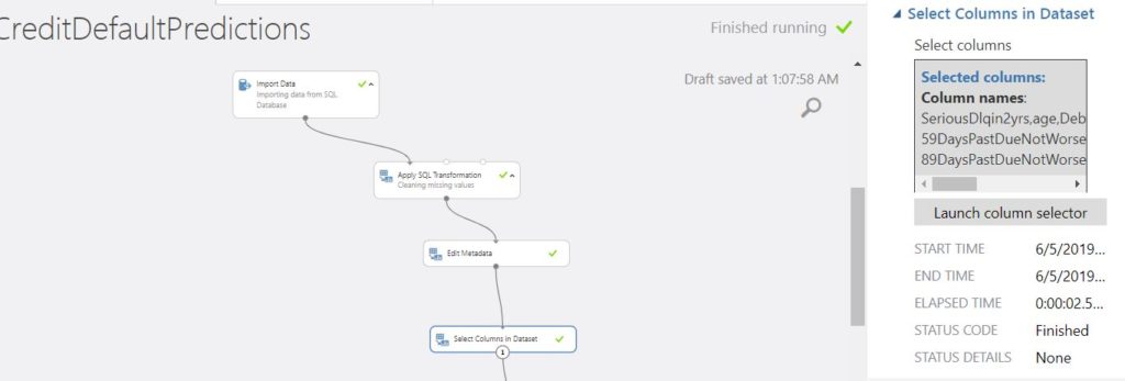
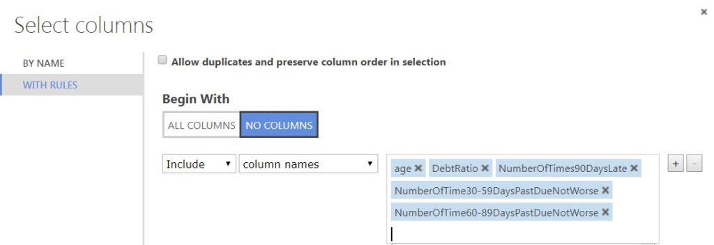
The primal aspect of predictive modeling is feature selection. Using rigorous statistical analysis, we select the features which correlate well with the label. Once we decide upon the features, we use the select columns in a dataset module to select the label and appropriate features.
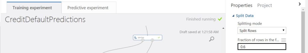
Further, we split the data into train and test set. The first set is used to train the model while the second one is used to test the same for metrics like accuracy.
Training
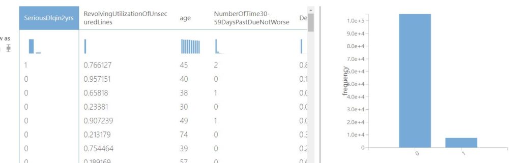
Now a primary visual analysis of the label column viz. SeriousDlqin2yrs reveals that it is unevenly distributed.
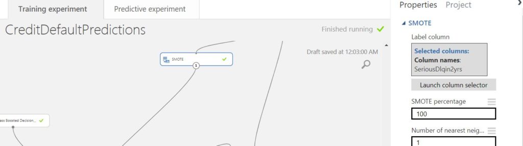
Training a predictive model is similar to teaching a child. If we train the model with one class disproportionately, the learning is skewed as well i.e. the model gets biased towards the majority class. As a result, there is a stark possibility that the model might misclassify the minority class as the majority class. To avoid this, we use a module named SMOTE. It is based on the concept of Synthetic minority over-sampling technique. Accordingly, this module oversamples the minority class by a certain factor, so that the model gets to learn all the classes proportionately. Please note that SMOTE should be applied only to the training set and not testing set. Also, select the label column to oversample as shown in the pic below.
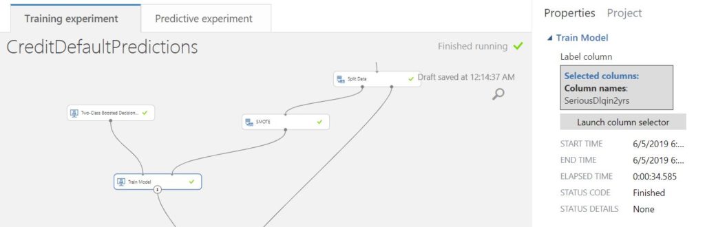
Next, use the Train Model module along with the algorithm of your choice. We will use the Two-Class Boosted Decision tree.
Testing
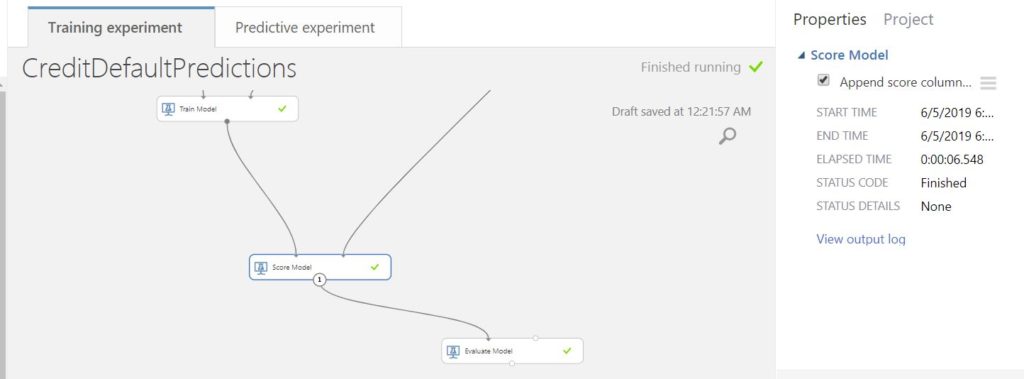
Once we are done with training the model, we need to score the model and evaluate its performance. Scoring and evaluation constitute the process of testing the model.
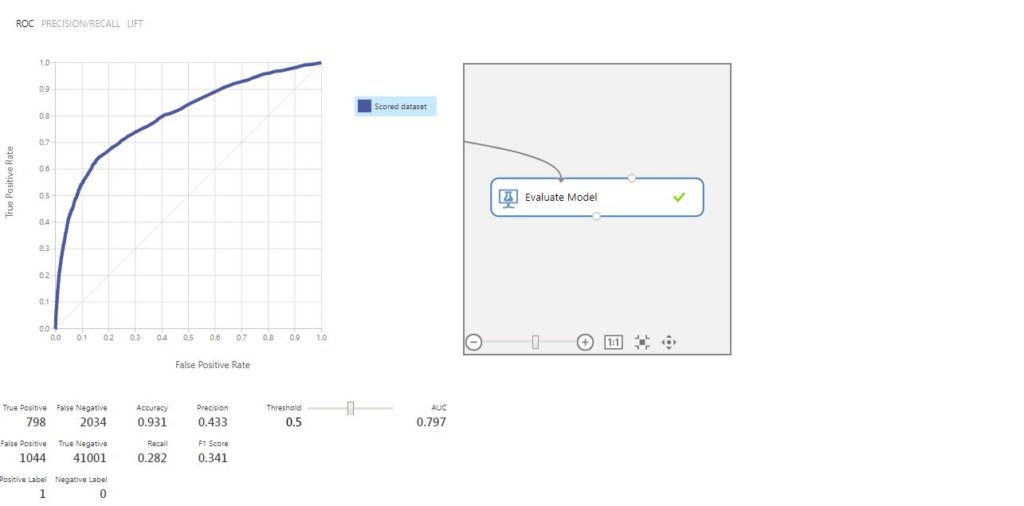
After running the entire experiment, we get the below ROC curve as the output of the Evaluate Model module.
Deployment
Now, after building a Machine Learning model, we intend to consume it in an application. In order to make it possible, we need to deploy the trained model. With Azure Machine Learning studio, it is a very easy and brisk process. Once the experiment is trained, click on the SETUP WEB SERVICE tab at the bottom and select Predictive Web Service. This creates a new Predictive Experiment with web service input and output. You need to make certain adjustments before you proceed with the further deployment process. Firstly, remove the label column from Select Columns in a dataset, since we won’t pass the label column as an input to the web service.
Secondly, change the point of connection to web service input from its original place to score model, since we pass correlated features as an input into the web service. Run the predictive experiment after this.
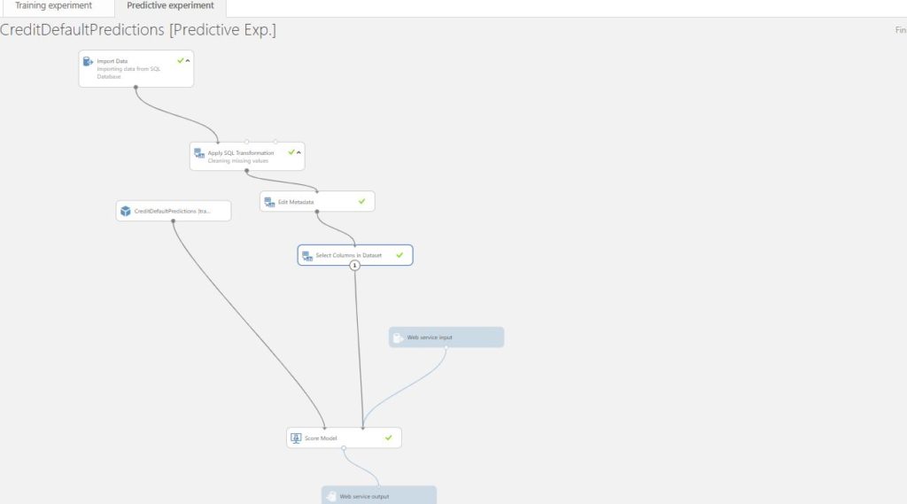
Finally, after running the experiment, deploy the web service(classic) as shown below.
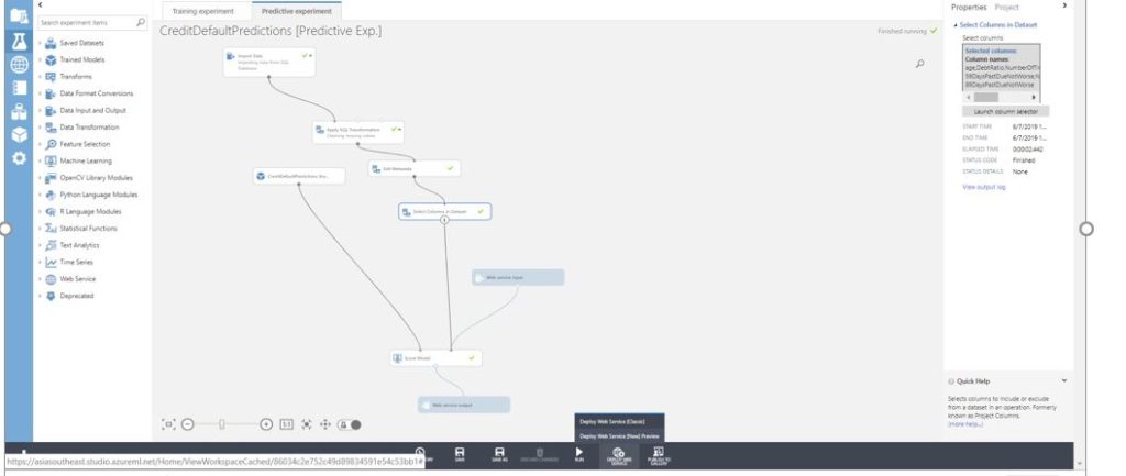
A new window opens up with details of the deployed web service. Next use the New Web Services Experience to test the endpoint.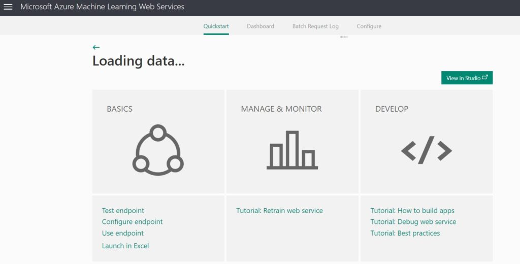
Clicking on the Test endpoint takes you to a web interface built by Microsoft to test your deployed model with sample data.
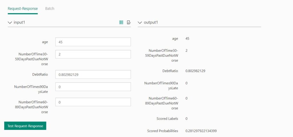
As evident from the above image, a person of a certain age (45) with some debt ratio and defaulter information, might not be a defaulter, going by the scored labels. In real life, such insights help businesses to plan their future course of action.
Conclusion
We hope that this article was useful and motivated an end to end Data Science process.
P.S.
- Ohm’s law image is from the following website: Ohms law experiment – Ohm’s law lab report
- Urea vs Osmotic pressure Image from the magoosh website: Urea in urine vs osmotic pressure
- Read this article to see anomaly detection in action for predictive maintenance: An Introduction to Azure IoT with Machine Learning. It uses Azure Machine Learning studio.
- Generally, the train-test split is in the ratio of 70:30.
Disclaimer: The articles and code snippets on data4v are for general information purposes only. We make no representations or warranties of any kind, express or implied, about the completeness, accuracy, reliability, suitability or availability with respect to the website or the information, products, services, or related graphics contained on the website for any purpose.